appliedprobability

Kelly’s Lemma

Kelly’s Lemma provides a way of using the time reversal of a Markov chain to calculate its stationary distribution. In theory, it is just a rewrite of the stationary distribution and time-reversal results for continuous-time chains. However, in application, it is different; you can take a guess at the time reversal of a chain $Q’$, and if you are right, i.e., if it checks out in Kelly’s Lemma, you get the stationary distribution as a consequence.

Stationary Distributions (Continuous Time)

We quickly recap the results known for discrete time that also hold in continuous time. (The slight advantage from a modeling perspective is that in continuous time, transitions occur distinctly, which gives more chances for reversibility to hold)

Continuous-time Markov chains

We want to model queueing systems in continuous time. Continuous-time Markov chains are a natural generalization of discrete-time Markov chains. We focus on developing intuition for continuous-time chains as the natural continuous-time extension of discrete chains, similar to our discussion of Poisson processes.

Poisson process

The Poisson process is a fundamental object in probability. Just as we have a uniform distribution for a single point in an interval, we would like a notion of a “uniform” distribution for a countable set of points in $\mathbb{R}$ . This motivates the Poisson process. We develop this intuition and then give a definition.

Stationary Distributions — Recap

We have characterized recurrence in terms of return times. However, if a Markov chain is positive recurrent, what proportion of time does it spend in each state?

Markov Chains Recurrence

We quickly recap the recurrence properties of Markov chains. The aim is to give a short review not a full rigorous treatment.

A discrete-time single-server queue

Many queues can be modeled as discrete-time Markov chains. Here, the state is the length of the queue, and fluctuations in arrivals and service give the random evolution from one time period to the next. Here is a diagram of a queue.

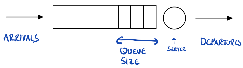
Figure: arrivals occur from the left and are stored in a buffer. Jobs or customers are represented as rectangles. A server is represented by a circle, which processes the jobs, and they then depart on the right-hand side.

Markov chains and matrices — A Quick Summary

Probabilities for a Markov chain can be expressed in terms of the probability vector $\boldsymbol{\lambda}$ and the transition matrix $P$ .

For example, for $x, x_0, \ldots, x_t \in \mathcal{X}$ and a function $r : \mathcal{X} \rightarrow \mathbb{R}$ ,

$\displaystyle \mathbb{P}(X_0 = x_0, \ldots, X_t = x_t) = \lambda_{x_0} P_{x_0 x_1} \cdots P_{x_{t-1} x_t}$

$\displaystyle \mathbb{P}(X_t = x) = [\lambda P^t]_x$

$\displaystyle \mathbb{E}_x[r(X_t)] = (P^t r)_x$

So essentially, multiplication to the left gives probabilities and multiplication to the right gives expectations.

Notation explanation. If the above is unclear, some notation may need explaining. For $P^t = P \times P \cdots \times P$ , we multiply $t$ copies of the matrix $P$ together.¹ Interpreting $\boldsymbol{\lambda}$ as a row vector, $\boldsymbol{\lambda} P^t$ is a row vector, and $[\boldsymbol{\lambda} P^t]_x$ is the $x$ -th component of that row vector.

Similarly, we can think of the function $r : \mathcal{X} \rightarrow \mathbb{R}$ as a column vector $\boldsymbol{r} = (r(x) : x \in \mathcal{X})$ . Then $P^t \boldsymbol{r}$ is a column vector under matrix multiplication, and $(P^t \boldsymbol{r})_x$ denotes its $x$ -th component.

Throughout these notes, $\mathbb{P}_x(\cdot) = \mathbb{P}(\cdot \mid X_0 = x)$ and $\mathbb{E}_x[\cdot] = \mathbb{E}[\cdot \mid X_0 = x]$ .

¹ We use $\top$ for transpose, not $t$ .

Discrete-time Markov chains — A Quick Look

Markov chains are the primary stochastic process used in queueing theory. The main elements of a Markov chain are its state and the independent randomness used to generate future states. This creates a very clean and natural form of dependence for which many properties are known. We will cover a few important properties of Markov chains, including recurrence, transience, and the existence of stationary distributions.

Zero-Order Stochastic Optimization: Keifer-Wolfowitz

We want to optimize the expected value of some random function. This is the problem we solved with Stochastic Gradient Descent. However, we assume that we no longer have access to unbiased estimate of the gradient. We only can obtain estimates of the function itself. In this case we can apply the Kiefer-Wolfowitz procedure.

The idea here is to replace the random gradient estimate used in stochastic gradient descent with a finite difference. If the increments used for these finite differences are sufficiently small, then over time convergence can be achieved. The approximation error for the finite difference has some impact on the rate of convergence.

Continue reading “Zero-Order Stochastic Optimization: Keifer-Wolfowitz”