The Law of Large Numbers and Central Limit Theorem

Let’s explain why the normal distribution is so important.

(This is a section in the notes here.)

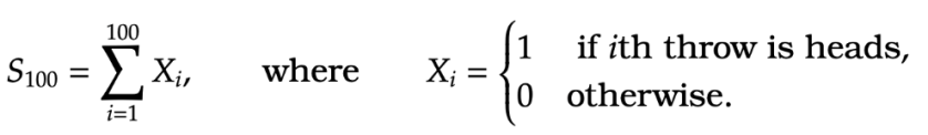
Suppose that I throw a coin $100$ times and count the number of heads $\begin{aligned} S_{100} = \sum_{i=1}^{100} X_i, \qquad \text{where} \qquad X_i = \begin{cases} 1 & \text{ if $i$th throw is heads},\\ 0 & \text{otherwise.} \end{cases} %\end{aligned}$

Screenshot 2021-11-18 at 16.35.48

The proportion of heads should be close to its mean $\begin{aligned} \frac{S_{100}}{100} \approx \frac{1}{2} = \mathbb E[X] \, %\end{aligned}$ and for $10,000$ it should be even closer. This can be shown mathematically (not just for coin throws but for quite general random variables)

Theorem [Weak Law of Large Numbers] For independent random variables $X_i$ , $i=1,...,n$ , with mean $\mu$ and variance bounded above by $\sigma$ , if we define

$S_n := \sum_{i=1}^n X_i$

then for all $\epsilon >0$

$\begin{aligned} \mathbb P\bigg( \mu - \epsilon \leq \frac{S_n}{n} \leq \mu + \epsilon \bigg) \xrightarrow[n\rightarrow \infty ]{} 1 \, .\end{aligned}$

We will prove this result a little later. But, continuing the discussion, suppose $X_1,...,X_n$ are independent identically distributed random variables with mean $\mu$ and variance $\sigma^2$ . We see from the above result that $S_n /n$ is getting close to $\mu$ . Nonetheless, in general, there is going to be some error. So let’s define

$\begin{aligned} \epsilon_n := \frac{S_n}{n} - \mu = \frac{S_n-n \mu}{n} \, .\end{aligned}$ So what does $\epsilon_n$ look like? We know that, in some sense, $\epsilon_n \rightarrow 0$ as $n \rightarrow \infty$ but how fast?

For this we can analyze the variance of the random variable $\epsilon_n$ : $\begin{aligned} \mathbb V( \epsilon_n) = \mathbb V \left( \frac{S_n-n \mu}{n} \right) =& \frac{1}{n^2} \mathbb V \left( S_n - n \mu \right) \notag \\ = & \frac{1}{n^2} \mathbb V \left( \sum_{i=1}^n (X_i - \mu) \right) \notag \\ = & \frac{1}{n^2} \sum_{i=1}^n \underbrace{ \mathbb V( X_i - \mu)}_{= \sigma^2} = \frac{\sigma^2}{n} %\end{aligned}$

Screenshot 2021-11-18 at 16.36.57

Thus the standard deviation of $\epsilon_n$ decreases as $\sigma / \sqrt{n}$ . Given this we can define $\begin{aligned} Z_n = \frac{\sqrt{n}}{\sigma} \epsilon_n = \frac{S_n - n \mu}{\sigma \sqrt{n}} \, . %\end{aligned}$

Screenshot 2021-11-18 at 16.37.18

Notice that $\mathbb E [Z_n]=0$ and $\begin{aligned} \mathbb V( Z_n) = \frac{n}{\sigma} \mathbb V(\epsilon_n) = 1. %\end{aligned}$

Screenshot 2021-11-18 at 16.37.22

So $Z_n$ has mean zero and its variance is fixed. I.e. the error as measured by $Z_n$ is not vanishing, but is staying roughly constant. So it seems like there is sometime happening for this random variable $Z_n$ , a question is what happens to $Z_n$ . The answer is that $Z_n$ converges to a normal distribution.

This is a famous and fundamental result in probability and statistics called the central limit theorem.

Theorem [Central Limit Theorem] For independent random variables $X_i$ with mean $\mu$ and variance $\sigma^2$ , for $S_n = \sum_{i=1}^n X_i$ and

$\begin{aligned} Z_n := \frac{S_n-n \mu}{\sigma \sqrt{n}}\end{aligned}$ then $\begin{aligned} \mathbb P (Z_n \leq z ) \xrightarrow[n \rightarrow \infty ]{} \mathbb P ( Z \leq z) %\end{aligned}$

Screenshot 2021-11-18 at 16.38.20

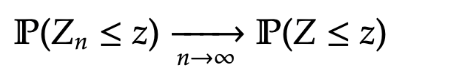
where $Z$ is a standard normal random variable.

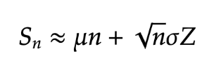
Given the discussion above the Central Limit Theorem, roughly says that $\begin{aligned} S_n \approx \mu n + \sqrt{n} \sigma Z %\end{aligned}$

Screenshot 2021-11-18 at 16.38.24

where $Z$ is a standard normal random variable. So whenever we measure errors about some expected value we should start to consider normal random variables.

Share this:

Leave a comment Cancel reply