Discrete-time Markov chains — A Quick Look

Markov chains are the primary stochastic process used in queueing theory. The main elements of a Markov chain are its state and the independent randomness used to generate future states. This creates a very clean and natural form of dependence for which many properties are known. We will cover a few important properties of Markov chains, including recurrence, transience, and the existence of stationary distributions.

Before getting into the details of discrete-time Markov chains (DTMCs), we quickly note that Markov chains can be discrete or continuous time. A key ingredient in the transition from discrete to continuous time is the Poisson process.

So before getting into queueing itself, we will cover:

Discrete-time Markov chains
Poisson processes
Continuous-time Markov chains

This is by no means an exhaustive list of Markovian processes. Other Markovian processes exist, such as Markov decision processes, renewal processes, and diffusion processes. These will be introduced as and when required.

To motivate the definition of a Markov chain, we will consider a simple example: the game of Snakes and Ladders. The game contains all the key elements of a Markov chain.

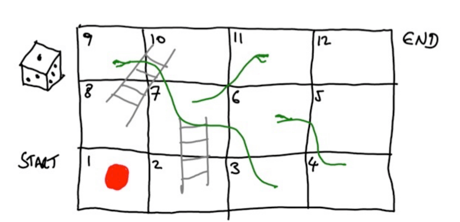
Figure: Snakes and ladders.

Recall that a player has a counter. (This is the red disk on square 1 in the figure above.) They throw a die. The number on the die determines how many spaces the counter moves. The aim is to get the counter from the start of the playing board to the end. The additional features are that if you land at the bottom of a ladder, you go to the top; and if you land on the head of a snake, you go to the tail. Players take turns until the end of the game.

The movement of the counter is a Markov chain. The key observations are:

The state is given by the position of the counter.
The next state is determined by:
1. The current state, that is, the current position of the counter;
2. The random throw of the die.

We can encapsulate the above observations into the following definition of a Markov chain.

Definition (Markov chain — a working definition).

A set of random variables $(X_t : t \in \mathbb{Z}_+)$ such that for $t \in \mathbb{Z}_+$

$\displaystyle X_{t+1} = f(X_t, U_t)$

where $U_t$ are IID random variables, is a Markov chain.

The above definition is not the standard definition of a Markov chain. In Snakes and Ladders, it is clear that $U_t$ should be the number on the die. It may not always be clear what $U_t$ should be for other processes. Also, this definition does not articulate an important property: the Markov property.

Snakes and Ladders and the Markov property

Let us consider the Snakes and Ladders game again to motivate a new definition. Suppose the counter is on square number 7, and let us consider what will happen next. For example, what is the probability that we move to square 10 next? It is $1/3$ : we can either throw a 3 or a 1 on the next die throw.

If you think about it, it does not matter how we arrived at the current state (square 7) in order to determine what happens next. Indeed, all that matters in deciding what happens in the future is that we are currently at square number 7, together with the future throws of the die. Thus, the past does not determine future states once we know the present state. This is called the Markov property.

Markov chain definition and the Markov property

Here is a broader definition, which considers the probabilities of different events rather than how random variables are generated.

Definition (Discrete-time Markov chain).

The stochastic process $(X_t : t \in \mathbb{Z}_+)$ is a Markov chain on a countable state space $\mathcal{X}$ when there is a matrix $P = (P_{xy} : x,y \in \mathcal{X})$ such that

$P_{xy} \geq 0$
$\sum_{y \in \mathcal{X}} P_{xy} = 1$

and there is a probability vector $\boldsymbol{\lambda} = (\lambda_x : x \in \mathcal{X})$ such that

$\displaystyle \begin{array}{rcl} \lambda_x & = & \mathbb{P}(X_0 = x_0) \\ P_{xy} & = & \mathbb{P}(X_{t+1} = x_{t+1} \mid X_t = x_t) \\ & = & \mathbb{P}(X_{t+1} = x_{t+1} \mid X_t = x_t, X_{t-1} = x_{t-1}, \ldots, X_0 = x_0) \end{array}$

for $x_0, x_1, x_2, \ldots \in \mathcal{X}$ .

The final equality above is the Markov property. Notice that in determining the future state $X_{t+1}$ , we can ignore the past states $X_{t-1}, \ldots, X_0$ provided we condition on the current state $X_t = x_t$ .