Conditional Probability

(This is a section in the notes here.)

Conditional probabilities are probabilities where we have assumed that another event has occurred.

An example: Two aces. Suppose we have a deck of cards and we consider the probability of getting an ace. If we take one card out, then the probability of an ace is $4/52 = 1/ 13$ . (There are $4$ aces in a pack of $52$ cards.) Now, given that the first card was an ace, we take a second card out the pack, notice now the probability of the second card being an ace has changed. Specifically there are now $3$ aces and $51$ cards in the pack. So the probability is $3/51=1/17$ . (Also observe that this probability is different than if we had assumed that the first card was not an ace, which in that case the probability would be $4/51$ .) Thus our condition on the first card has effected the probability for the second card. This is an example of conditional probability, which we now develop more generally.

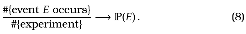
Motivating a definition of conditional probability. Recall that we thought of probability as $\begin{aligned} \frac{\# \{\text{event $E$ occurs}\} }{ \# \{\text{experiment}\}} \longrightarrow \mathbb P(E)\, . \label{probconv2} %\end{aligned}$

Screenshot 2021-11-18 at 15.03.33

Similarly, as we think of conditional probability as the proportion of time that an event occurs knowing that an other event has occurred. In this case, an analogous statement would be that $\begin{aligned} \label{probcond} \frac{\# \{ \text{event B and event A occur}\}}{\# \{ \text{event A occurs}\}} \longrightarrow \mathbb P(B|A)\, . %\end{aligned}$

Screenshot 2021-11-18 at 15.04.01

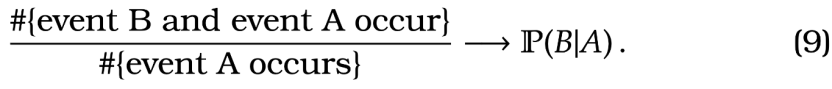
where here we use $\mathbb P(B|A)$ to denote the probability of event $B$ conditional on event $A$ .

Observe, that we can express (9) in terms of (8). In particular, $\begin{aligned} \label{probcond2} & \frac{\# \{ \text{event B and A occur}\}}{\# \{ \text{event A occurs}\}} \notag = \frac{\displaystyle \frac{\# \{\text{event B and A occur}\} }{ \# \{\text{experiment}\}}}{ \displaystyle \frac{\# \{\text{event A occurs}\} }{ \# \{\text{experiment}\}}} \longrightarrow \frac{\mathbb P (A \cap B)}{\mathbb P( A)} %\end{aligned}$

Screenshot 2021-11-18 at 15.04.12

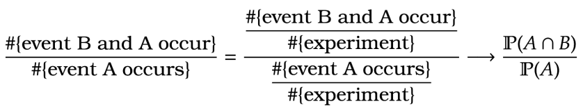
Here we divide the denominator and numerator from the left hand side of by the number of experiments and then we apply to both expressions.

This motivates the following

Screenshot 2021-11-18 at 15.05.32

Definition of conditional probability. Given the above we have:

Definition [Conditional Probability] For events $A$ and $B$ , the conditional probability of $B$ given $A$ is $\begin{aligned} \mathbb P (B| A ) := \frac{ \mathbb P ( A \cap B) }{ \mathbb P(A) } %\end{aligned}$

Screenshot 2021-11-18 at 15.05.32

when $\mathbb P(A)>0$ . By convention, if $\mathbb P(A) =0$ then we define $\mathbb P(B|A) = 0$ .

A couple of examples.

Example. The results of a survey of 250 different 75 year-olds is given in the following Venn diagram.

Screenshot 2021-11-18 at 15.06.31

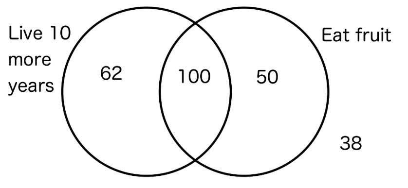
For a randomly selected participant in the survey:

1) Calculate the probability living 10 more years given that they eat fruit.

2) Calculate the probability living 10 more years given that they don’t eat fruit.

Answer. 1) $\begin{aligned} \mathbb P ( \text{ live 10 years } | \text{ eat fruit })= \frac{100}{100 +50} = 0.667 %\end{aligned}$

Screenshot 2021-11-18 at 15.07.29

2) $\begin{aligned} \mathbb P ( \text{ live 10 years } | \text{ don't eat fruit })= \frac{62}{62+38} = 0.62 %\end{aligned}$ So you should eat fruit…

Screenshot 2021-11-18 at 15.07.35

Example. I have two siblings, given I have a brother, what is the probability that I also have a sister.

Answer. Note that our sample space is $\Omega = \{BB,BS,SB,SS\}$ . E.g. here $BS$ means the eldest sibling is a brother and the youngest is a sister. Each outcome has equal probability of $1/4$ . So $\begin{aligned} \mathbb P ( \text{ sister } | \text{ brother } ) = \frac{ \mathbb P (BS) + \mathbb P(SB) }{\mathbb P(BB)+\mathbb P (BS) + \mathbb P(SB)} = \frac{2/4}{3/4} = \frac{2}{3} %\end{aligned}$

Screenshot 2021-11-18 at 15.08.22

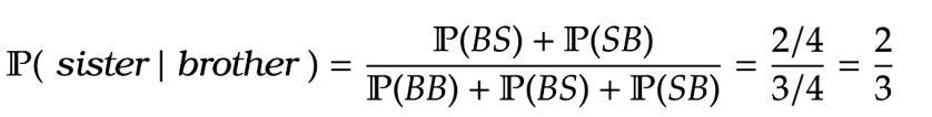
For some this is an example of conditional probability being a bit counter-intuitive, as ones gut reaction is that the answer is a half. Notice if I specified that my eldest sibling was a brother then the answer would indeed be a half. This is just one small example of the subtle art of manipulating conditional probabilities.

Independence

We are interested in the setting where knowing that an event has occurred does not affect another event. E.g. if I roll a dice twice, in principle the outcome of the first roll should not influence the second roll. If event $A$ does not influence event $B$ then it should be that $\begin{aligned} \mathbb P( B | A ) = \mathbb P(B) %\end{aligned}$

Screenshot 2021-11-18 at 15.09.11

I.e. conditioning on $A$ having happened does not change the probability of $B$ occuring. Since $\mathbb P (B | A) = \mathbb P (A \cap B)/\mathbb P( A)$ , we can slightly more symmetrically express the above equality as $\begin{aligned} \mathbb P(A \cap B) = \mathbb P (A) \times \mathbb P(B)\, . %\end{aligned}$

Screenshot 2021-11-18 at 15.09.14

This is what we call independence of two events.

Definition [Independence] We say that events $A$ and $B$ are independent if $\begin{aligned} \mathbb P( A \cap B) = \mathbb P(A) \mathbb P(B) \,. %\end{aligned}$

Screenshot 2021-11-18 at 15.09.14

So if knowing that $A$ has happened does not affect the probability of $B$ then we multiply the probabilities together.

Warning! The following is sometimes confused by students. We say that two events are “mutually exclusive” if $A \cap B = \emptyset$ . In that case we know from Lemma [lem:op1] that we add the probabilities together. This not the same as independence where we multiply the probabilities together.

As discussed, independence says that knowing an outcome is in $A$ does not effect the probability of $B$ . However, if events $A$ and $B$ are mutually exclusive, then knowing the outcome is in $A$ effects the probability of $B$ . Specifically, if we know an outcome is in $A$ then it definitely is not in $B$ .

Example. What is the probability of getting $10$ heads in a row from an unbiased coin?

Answer. Since with multiple probabilities together $\begin{aligned} \mathbb P( HHHHHHHHHH) &= \mathbb P(H) \mathbb P(H) \mathbb P(H) \mathbb P(H) \mathbb P(H) \mathbb P(H) \mathbb P(H) \mathbb P(H) \mathbb P(H) \mathbb P(H) \\ & = \bigg(\frac{1}{2}\bigg)^{10} = \frac{1}{1024} \,. %\end{aligned}$

Screenshot 2021-11-18 at 15.11.10

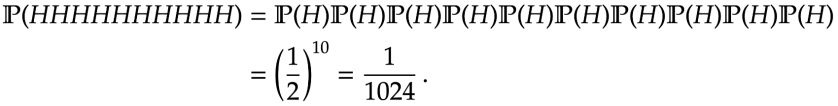
This is actually a “magic trick”. Notice there are $1440$ minutes in a day. So enough time to have a reasonable chance of getting $10$ heads in a row over the course of a day. There are TV magicians that had performed this as a trick (by cutting out the roughly $1023$ previous camera takes).

Rules for Conditional Probabilities

Here are few useful formulas for Conditional Probabilities. (Like with operations on sets the proofs are not entirely necessary to know for exams.)

Lemma 1.

$\mathbb P (A \cap B) = \mathbb P ( B | A ) \mathbb P(A)$

Proof. Follows immediately from the definition of $\mathbb P(B|A)$ . $\square$ .

This is useful as it can be easier to find $\mathbb P(B|A)$ . E.g. like with the earlier two aces example, we can easily find the probability of drawing a ace from a deck given the previous card was an ace, and from that calculate the probability of two aces.

Lemma 2.

$\mathbb P(B) = \mathbb P(B | A ) \mathbb P(A)+ \mathbb P (B | A^c) \mathbb P(A^c)$

Proof. Since $B = (A \cap B) \cup (A^c \cap B)$ , then Lemma 1 gives

Screenshot 2021-11-18 at 15.13.11

$\begin{aligned} \mathbb P ( B ) = \mathbb P(B \cap A ) + \mathbb P(B \cap A^c) %\end{aligned}$ and then applying Lemma 1

$\mathbb P(B) = \mathbb P(B | A ) \mathbb P(A)+ \mathbb P (B | A^c) \mathbb P(A^c)$

gives $\begin{aligned} \mathbb P ( B ) = \mathbb P(B | A ) \mathbb P(A) + \mathbb P(B | A^c) \mathbb P(A^c) %\end{aligned}$ as required. $\square$

Note that the above result can be applied to any number of sets $A_1,...,A_n$ . So long as $\cup_i A_i = \Omega$ and $A_i \cap A_j = \emptyset$ for $i \neq j$ , it holds that $\begin{aligned} \mathbb P (B ) = \sum_{i=1}^n \mathbb P( B | A_i) \mathbb P(A_i)\, . %\end{aligned}$

Screenshot 2021-11-18 at 15.13.50

Lemma 3 [Bayes’ Rule] $\begin{aligned} \mathbb P (B |A ) = \frac{\mathbb P(A | B ) \mathbb P(B) }{\mathbb P(A)} %\end{aligned}$

Screenshot 2021-11-18 at 15.14.42

The result is sometimes called Bayes’ Theorem, as well.

$\begin{aligned} \mathbb P ( B | A ) = \frac{\mathbb P(A \cap B)}{\mathbb P(A) } = \frac{\mathbb P ( A \cap B) }{ \mathbb P(B)} \frac{ \mathbb P (B) }{ \mathbb P (A) } = \frac{\mathbb P (A | B ) \mathbb P(B)}{\mathbb P(A)} \, . %\end{aligned}$ Screenshot 2021-11-18 at 15.15.32

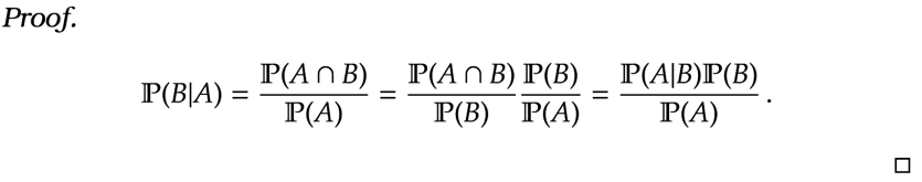
Bayes’ Rule reverses the order of the conditional probability. There is a whole branch of statistics developed to this which we will very briefly touch upon shortly.

Example [Two aces] Taking out two cards from a well-shuffled deck. What is the probability that both cards are aces? What is the probability that the 2nd card is an ace?

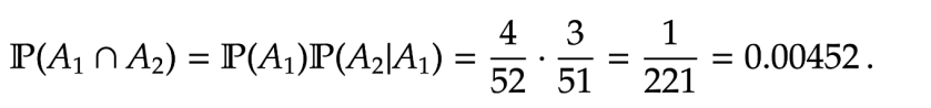
Answer. We know that $\mathbb P(A_1) = {4}/{52}$ . Also we know that $\mathbb P (A_2 | A_1 ) = {3}/{51}$ , because after one ace is dealt then there are $3$ aces and $51$ cards. Thus using Lemma 1

Screenshot 2021-11-18 at 15.16.27 $\begin{aligned} \mathbb P (A_1 \cap A_2) = \mathbb P(A_1) \mathbb P( A_2 |A_1) = \frac{4}{52} \cdot \frac{3}{51} = \frac{1}{221} = 0.00452 \, . %\end{aligned}$ For the 2nd part, we can apply Lemma 7. Here $\begin{aligned} \mathbb P ( A_2) & = \mathbb P ( A_2 | A_1 ) \mathbb P(A_1) + \mathbb P(A_2 | A_1^c) \mathbb P(A_2^c) \\ & = \frac{4}{52} \cdot \frac{3}{51} + \frac{48}{52} \cdot \frac{4}{51} = \frac{1}{13} . %\end{aligned}$

Screenshot 2021-11-18 at 15.16.32

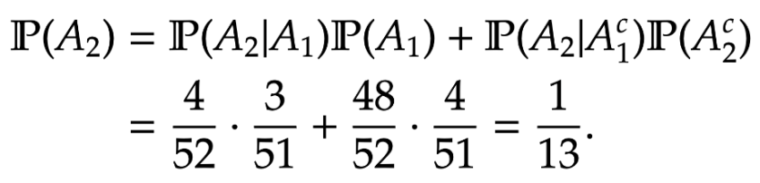
This should come as no surprise, as the probability that the 2nd card is an ace should be the same as the probability that the 1st card is an ace. (Imagine taking the first card out the pack and putting it to the back, and then taking the 2nd card out and looking at it.)

Example [Frequentist vs Bayesian Statistics] I have a biased coin, it is biased so the probability of heads, $\theta$ , is either $3/4$ or $1/4$ , but you don’t know which. So you throw the coin three times and get three heads. From this data determine if $\theta = 3/4$ or $\theta = 1/4$ .

Answer. This is clearly not a well-defined question, because we cannot determine with certainty the value of $\theta$ . Given it’s subjective nature (where there is no right answers). We give two approaches: a frequentist approach, which is a more classical statistical approach, and a bayesian statistical approach.

The Frequentist Answer. The likelihood of three heads for both choices of $\theta$ is

$\begin{aligned} \mathbb P ( HHH | \theta = {1}/{4} ) = \left( \frac{1}{4} \right)^3 \quad \text{and} \quad % \mathbb P ( HHH | \theta = {3}/{4} ) = \left( \frac{3}{4} \right)^3\, .\end{aligned}$ The parameter that gives the highest probability is $\hat \theta= {3}/{4}$ . So our answer for this problem is the estimator $\hat \theta = 3/4$ .

The Bayesian Answer. Since we don’t know in prior to throwing the coin, which of the two possibilities hold. We could give each possibility equal likelihood that is $\begin{aligned} \mathbb P ( \theta = 1/4) = \mathbb P ( \theta = 3/4) = \frac{1}{2} %\end{aligned}$

Screenshot 2021-11-18 at 15.18.30

This is called the prior distribution. After throwing the coin and getting three heads then we want to update our estimate to find $\begin{aligned} \mathbb P ( \theta = 1/4 | HHH) \quad \text{and} \quad \mathbb P ( \theta = 3/4 | HHH) %\end{aligned}$

Screenshot 2021-11-18 at 15.18.35

This called the posterior distribution. We can use Bayes’ Rule to calculate the posterior: $\begin{aligned} \mathbb P ( \theta = 3/4 | HHH) & = \mathbb P ( HHH | \theta = 3/4) \frac{\mathbb P ( \theta = 3/4) }{ \mathbb P (HHH) } \notag \\ & = \left( \frac{3}{4} \right)^3 \frac{\frac{1}{2} }{ \mathbb P (HHH)} \label{Bayes1} %\end{aligned}$

Screenshot 2021-11-18 at 15.18.48

To calculate $\mathbb P (HHH)$ we can apply Lemma 2

$\begin{aligned} \mathbb P (HHH) =& \mathbb P ( HHH | \theta = 3/4) \mathbb P (\theta = 3/4) + \mathbb P ( HHH | \theta = 1/4) \mathbb P (\theta = 1/4) \notag \\ = & \left( \frac{3}{4} \right)^3 {\frac{1}{2} } + \left( \frac{1}{4} \right)^3 {\frac{1}{2} } =\frac{28}{128}\end{aligned}$ which then gives with (10) that

Screenshot 2021-11-18 at 15.20.15

and thus $\mathbb P ( \theta = 1/4 | HHH) = \frac{1}{28}$ . Thus in the Bayesian approach we says that we think $\theta = 3/4$ with probability $27/28$ .

Under reasonable assumptions and enough data both the Bayesian and Frequentist approaches will converge on the correct parameter. The choice of the prior in the Bayesian approach is quite subjective. When the range of parameters gets large (or continuous) then we need to solve an optimization problem in the frequentist approach, while in the Bayesian approach we need to sum over a large number of terms to find the normalizing constant, which was the $\mathbb P(HHH)$ term in the above example.