Often we are interested in the magnitude of an outcome as well as its probability. E.g. in a gambling game amount you win or loss is as important as the probability each outcome.

(This is a section in the notes here.)

Definition [Random Variable] A random variable is a function $X : \Omega \rightarrow \mathbb R$ that gives a value for every outcome in the sample space.

For example, if we roll two dice then $\Omega = \{ (d_1,d_2): d_1,d_2 \in \{1,2,3,4,5,6 \}\}$ is our sample space and the sum of the two dice can be given by $X((d_1,d_2)) = d_1+d_2$ .

Random variables (RVs) can be discrete, e.g. taking values $1,2,3,...$ , or they can be continuous, e.g. taking any value in $\mathbb R$ .

Typically we use capital letters to denote random variables $X,Y,Z$ . Often we suppress the underlying sample space when writing probabilities. E.g. for our sum of two dice examples, we might write $\begin{aligned} \mathbb P( X = 2) = \frac{1}{36} \, , %\end{aligned}$

Screenshot 2021-11-18 at 15.26.04

where here by $\{ X =2 \}$ we really mean the event $\{ \omega \in \Omega : X(\omega) =2 \}$ .

Discrete Probability Distributions. A key way to characterize a random variable is with its distribution.

Definition [Probability Mass Function]The probability distribution of a discrete random variable $X$ with values in the finite or countable set $\mathcal X \subseteq \mathbb R$ is given by

Screenshot 2021-11-18 at 15.26.56

$\begin{aligned} p(x) = \mathbb P(X=x), \qquad x \in \mathcal X\, . %\end{aligned}$ This is some times called the probability mass function (PMF). Notice it satisfies the properties

(Positive) For all $x \in \mathcal X$ ,

$p(x) \geq 0$

(Sums to one) $\sum_{x \in \mathcal X} p(x) = 1\, .$

Another way to characterize the distribution of the a random variable is through its cumulative distribution function, which is simply gives the probability that the random variable is below a given value.

Definition [Cumulative Distribution Function] The cumulative distribution function (CDF) of a random variable $X$ is

$\begin{aligned} F_X(x) := \mathbb P( X \leq x)\, , \end{aligned}$ $x \in \mathbb R$ .

We can define more than one random variable on the same probability space. E.g. from our two dice throws, $X$ could be the value of first dice, $Y$ could be the value of the second dice, and $Z$ could be the sum of the two dice.

Definition [Joint Probability Distribution] Suppose there are two random variables defined on the same probability space, $X: \Omega \rightarrow \mathcal X \subseteq \mathbb R$ and $Y: \Omega \rightarrow \mathcal Y \subseteq \mathbb R$ , then the joint probability mass function is given by $\begin{aligned} p(x,y):= \mathbb P ( X = x, Y= y), %\end{aligned}$

Screenshot 2021-11-18 at 15.27.54

for $x \in \mathcal X$ and $y \in \mathcal Y$ .

Definition [Independent Random Variables] We say that $X$ and $Y$ are independent random variables if $\begin{aligned} \mathbb P(X=x, Y=y) = \mathbb P(X=x) \cdot\mathbb P(Y=y) %\end{aligned}$

for all $x \in \mathcal X$ , $y \in \mathcal Y$ (I.e. $p(x,y) = p_X(x) p_Y(y)$ ).

We can extend the about definition to any number of random variables. E.g. a set of random variable $X_1,X_2,X_3,...,X_n$ are independent if $\begin{aligned} \mathbb P( X_1= x_1,...,X_n=x_n) = \prod_{i=1}^n \mathbb P(X_i = x_i) \, . %\end{aligned}$

Screenshot 2021-11-18 at 15.28.50

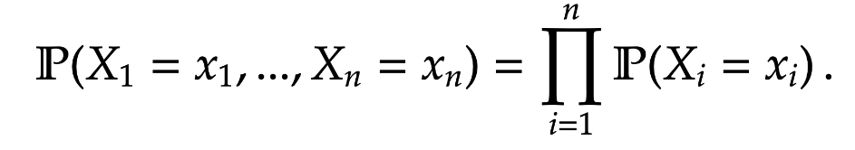
A common situtation that we are interested in is where $X_1,...,X_n$ are independent identically distributed random variables or IIDRVs, for short. Here in addition to being independent, the random variables each have the same CDF. Here we think of IIDRVs repeating the same random experiment $n$ times and recording the answer to each.

Expectation and Variance

Definition. The expectation of a discrete random variable $X$ is $\begin{aligned} \mathbb E [ X] = \sum_{x \in \mathcal X} x \cdot \mathbb P(X=x) \, . %\end{aligned}$

Screenshot 2021-11-18 at 15.29.19

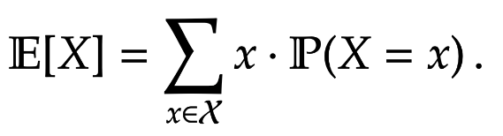
The expectation gives an average value of the random variable. We could think of placing one unit of mass along the number line, where at point $x$ we place a weight of $\mathbb P(X=x)$ . The expectation, $\mathbb E[X]$ , is then the point of the number line that balances the weights on the left with the right.

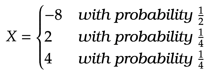
Example. Calculate the expectation for the following random variable $\begin{aligned} X = \begin{cases} -8 & \text{with probability } \frac{1}{2} \\ 2 & \text{with probability } \frac{1}{4} \\ 4 & \text{with probability } \frac{1}{4} \end{cases}\end{aligned}$

Screenshot 2021-11-18 at 15.30.21

Answer.

$\begin{aligned} \mathbb E [ X] = -8 \times \frac{1}{2} + 2 \times \frac{1}{4} + 4 \times \frac{1}{4} = - 2 \tfrac{1}{2} \, .\end{aligned}$

Properties of the expectation

Here are various properties of the expectation. Proofs are included and are good to know but are not essential reading for exams. (For the most part the following lemmas are really properties of summation.)

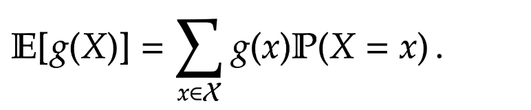
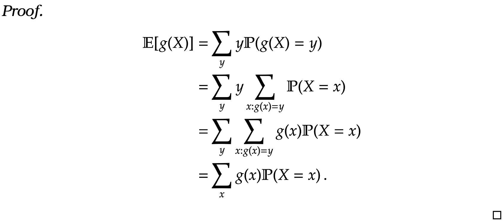
Lemma 1. For a function $g: \mathcal X \rightarrow \mathbb R$ , $\begin{aligned} \mathbb E [ g(X) ] = \sum_{x \in \mathcal X} g(x) \mathbb P(X=x) \, . %\end{aligned}$

Screenshot 2021-11-18 at 15.31.18 $\begin{aligned} \mathbb E [ g(X) ] =& \sum_y y\mathbb P(g(X) = y) \notag \\ = & \sum_y y \sum_{x : g(x) =y } \mathbb P(X=x) \notag \\ = & \sum_y \sum_{x : g(x) = y} g(x) \mathbb P (X =x) \notag \\ = & \sum_x g(x) \mathbb P(X=x) \, . %\end{aligned}$

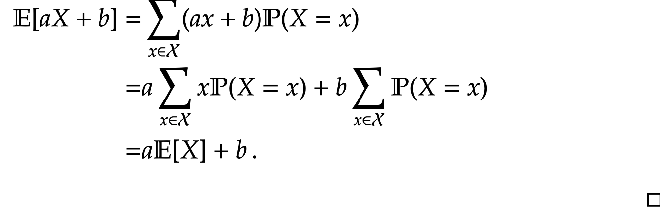
Lemma 2. For constants $a$ and $b$ $\begin{aligned} \mathbb E [ a X + b ] = a \mathbb E [ X] + b %\end{aligned}$

Screenshot 2021-11-18 at 15.32.19

Proof. Applying Lemma 1.

Screenshot 2021-11-18 at 15.33.50

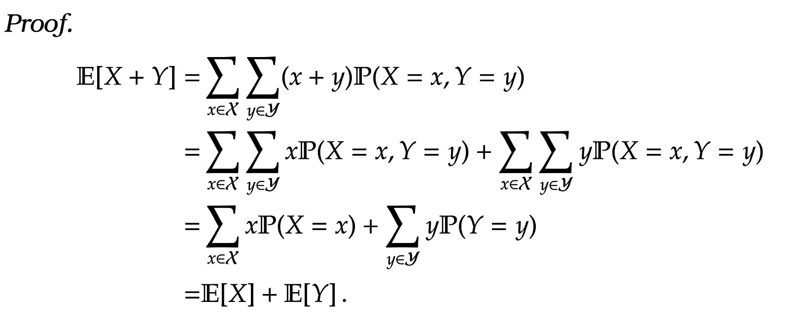
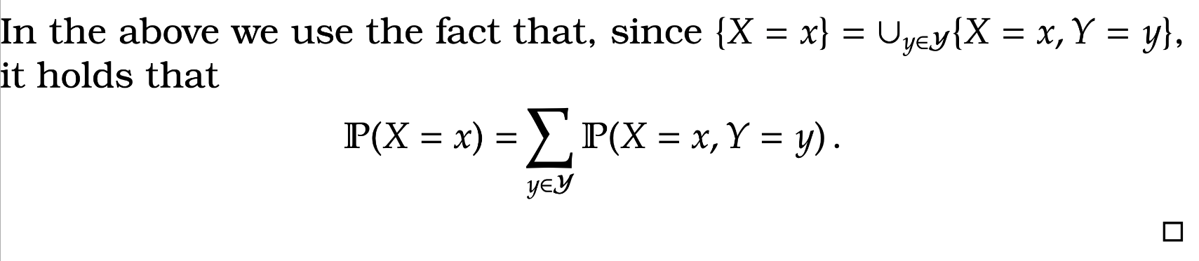
Lemma 3. For two random variables $X$ and $Y$ $\begin{aligned} \mathbb E [ X + Y ] = \mathbb E [ X ] + \mathbb E[Y] \, . %\end{aligned}$

Screenshot 2021-11-18 at 15.34.18 $\begin{aligned} \mathbb E [ X + Y ] = & \sum_{x \in \mathcal X} \sum_{y \in \mathcal Y} ( x+ y ) \mathbb P(X=x, Y=y) \notag \\ = & \sum_{x \in \mathcal X} \sum_{y \in \mathcal Y} x \mathbb P(X=x, Y=y) + \sum_{x \in \mathcal X} \sum_{y \in \mathcal Y} y \mathbb P(X=x, Y=y) \notag \\ = & \sum_{x \in \mathcal X} x \mathbb P(X=x) + \sum_{y \in \mathcal Y} y \mathbb P(Y=y) \notag \\ = & \mathbb E[X] + \mathbb E[Y]\, . %\end{aligned}$

Screenshot 2021-11-18 at 15.34.45

Screenshot 2021-11-18 at 15.34.56

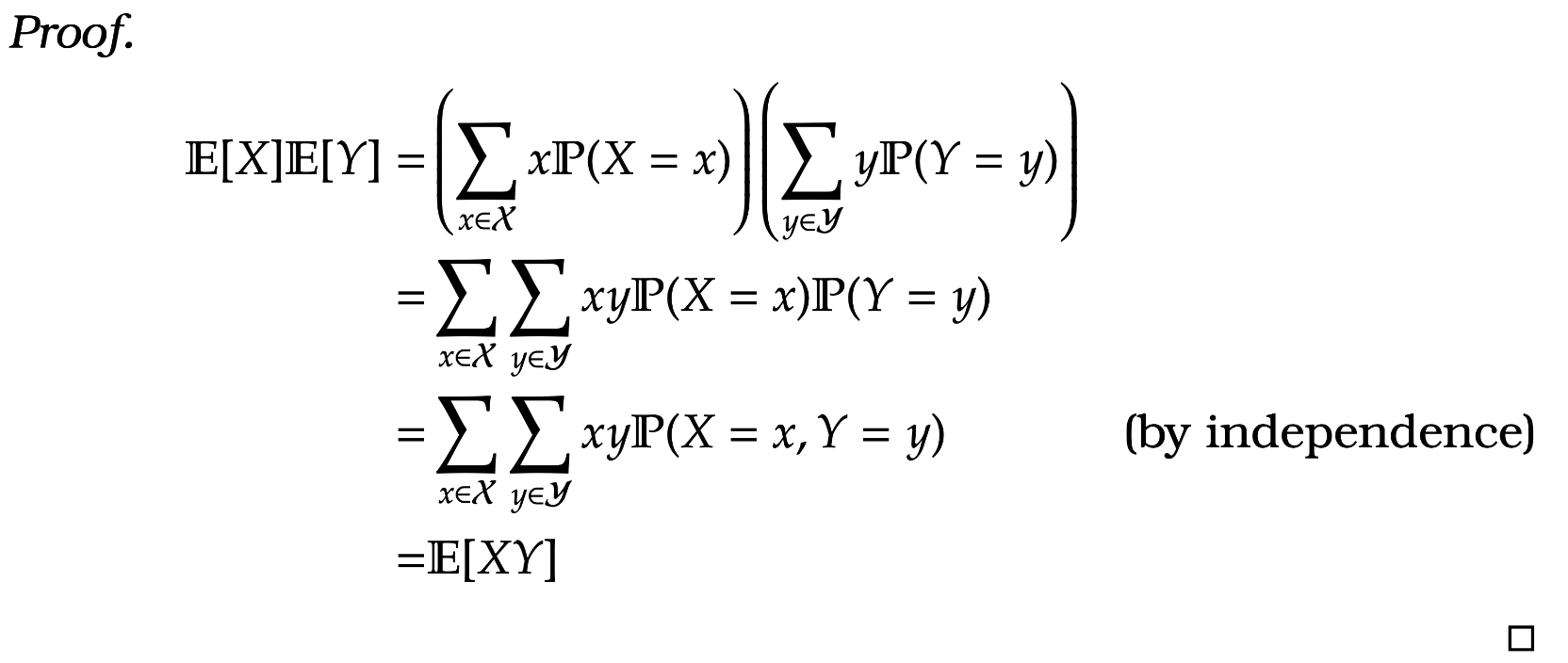
Lemma 4. For two independent random variables $X$ and $Y$ $\begin{aligned} \mathbb E [ X\cdot Y ] = \mathbb E [ X ] \cdot \mathbb E[Y] \, . %\end{aligned}$

Screenshot 2021-11-18 at 15.35.54

Warning! In general, we cannot multiply expectations in this way. We need independence to hold. For instance if $X=Y =1$ with probability $1/2$ and $X=Y=0$ otherwise a quick check shows that $1/2 = \mathbb E [ X Y] \neq \mathbb E[X] \mathbb E[Y] = 1/4$ .

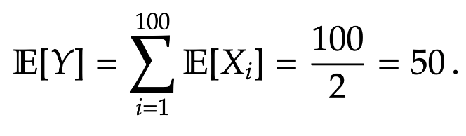
Example. Let $Y$ the number of heads from $100$ coin tosses then $\mathbb E [Y] = 50$ .

Answer. The exact distribution of $Y$ is not so straight-forward to explicitly calculate. However, we can use the above rules.

Note that $Y = \sum_{i=1}^{100} X_i$ where

$\begin{aligned} X_i = \begin{cases} 1, & \text{if $i$th coin is heads},\\ 0, & \text{otherwise.} \end{cases}\end{aligned}$

It is easy to see that $\mathbb E[X_i ] = 1 \mathbb P(X_i =1 ) + 0 \mathbb P(X_i = 0) = 1/2$ . Thus by Lemma 3

Screenshot 2021-11-18 at 15.36.59

Variance

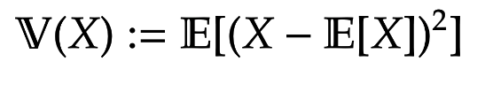
While the expectation gives an average value for a random variable. The variance determines how spread out a probability distribution is.

Definition [Variance / Standard Deviation] The variance of a random variable $X$ is defined to be $\begin{aligned} \mathbb V(X) := \mathbb E[ (X- \mathbb E[X])^2] %\end{aligned}$

Screenshot 2021-11-18 at 15.37.42

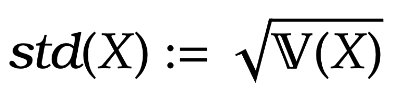
Further the standard deviation is the square-root of the variance. That is $\begin{aligned} \text{std} (X) := \sqrt{ \mathbb V(X)} %\end{aligned}$

Screenshot 2021-11-18 at 15.37.45

It is common to use $\mu$ to denote the expectation of a random variable and for $\sigma$ to denote the variance of a random variable. So $\begin{aligned} \sigma^2 = \mathbb E[ (X- \mu)^2 ] \, . %\end{aligned}$

Screenshot 2021-11-18 at 15.38.14

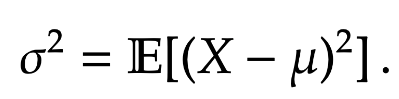
Here we use $(X-\mu)^2$ to determine a square distance about the mean. We then take the square root to give the rescale the distance. This is very similar to the way we think of (Euclidean) distances for vectors, E.g. for $x = (x_1,x_2)$ , $| x| = \sqrt{x_1^2+x_2^2}$ .

Lemma 5.

Screenshot 2021-11-18 at 15.38.55

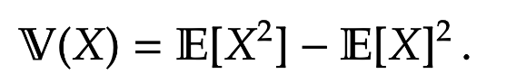
So the variance is the mean square minus the square of the mean.

Proof.

$\begin{aligned} \mathbb V(X) = & \mathbb E [ (X- \mathbb E[X])^2 ] \notag \\ = & \mathbb E [ X^2 - 2 X \mathbb E[X] + \mathbb E[X]^2 ] \notag \\ = & \mathbb E[X^2 ] - 2 \mathbb E[X] \mathbb E[X] + \mathbb E[X]^2 \notag \\ = & \mathbb E[ X^2] - \mathbb E[X]^2 \, .\end{aligned}$

$\square$

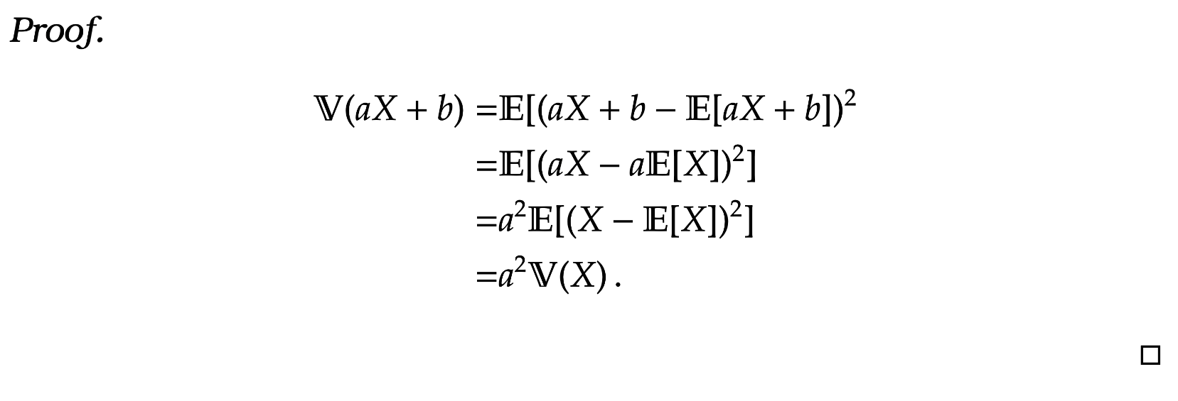
Lemma 6. For $a,b \in \mathbb R,$

$\begin{aligned} \mathbb V( a X + b ) = a^2 \mathbb V(X) \, .\end{aligned}$

$\begin{aligned} \mathbb V(a X + b) = & \mathbb E[ ( a X + b - \mathbb E[ a X +b ])^2 \notag \\ = & \mathbb E[ (a X - a \mathbb E[X])^2 ] \notag \\ = & a^2 \mathbb E[ (X- \mathbb E[X])^2 ] \notag \\ = & a^2 \mathbb V(X) \, . %\end{aligned}$ Screenshot 2021-11-18 at 15.39.59

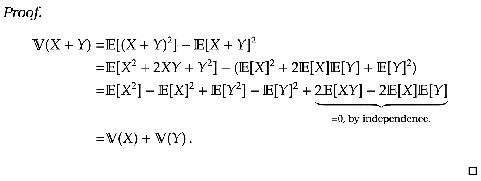
Lemma 7. If $X$ and $Y$ are independent random variables then $\begin{aligned} \mathbb V(X + Y) = \mathbb V(X) + \mathbb V(Y)\, . %\end{aligned}$

$\begin{aligned} \mathbb V(X+Y) = & \mathbb E[ (X+Y)^2 ] - \mathbb E [X+Y]^2 \notag \\ = & \mathbb E[ X^2 + 2XY + Y^2 ] - ( \mathbb E[X]^2 + 2 \mathbb E[X] \mathbb E[Y] + \mathbb E[Y]^2 ) \notag \\ = & \mathbb E[ X^2] - \mathbb E[X]^2 + \mathbb E[Y^2] - \mathbb E[Y]^2 + \underbrace{2 \mathbb E[ XY] - 2 \mathbb E[X] \mathbb E[Y]}_{=0, \text{ by independence.}} \notag \\ = & \mathbb V(X) + \mathbb V(Y) \,. %\end{aligned}$ Screenshot 2021-11-18 at 15.40.36

Notice if we have a sequence of independent identically distributed random variables (IIDRVs) $X_1,....,X_n$ where $\mathbb V(X_1) = \sigma^2$ then we can see from the above lemma that $\begin{aligned} \text{std}\bigg( \sum_{i=1}^n X_i \bigg) = \sqrt{ \mathbb V\bigg( \sum_{i=1}^n X_i \bigg) } = \sqrt{\sum_{i=1}^n \mathbb V\big( X_i \big) } = \sigma\sqrt{n} \,. %\end{aligned}$

Screenshot 2021-11-18 at 15.41.08

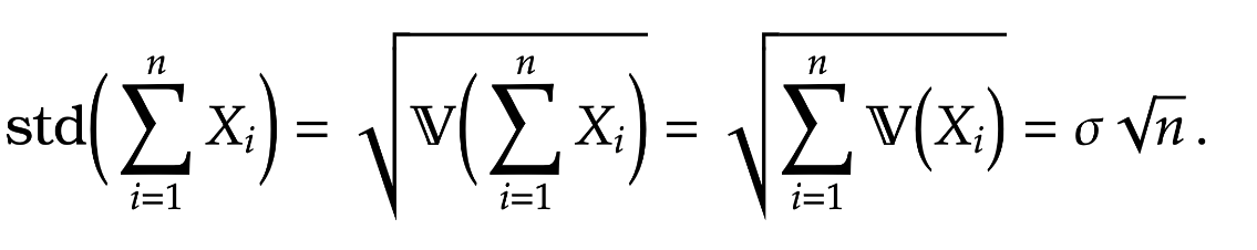
So we see that as we add up more and more IIDRVs the distance from the mean is about $\sqrt{n}$ . This is an important observation that will be refined later on where we discuss the normal distribution.

Random Variables and Expectation

Expectation and Variance

Properties of the expectation

Variance

Leave a Reply Cancel reply

Expectation and Variance

Properties of the expectation

Variance

Share this:

Like this:

Leave a Reply Cancel reply