(This is a section in the notes here.)

I throw a coin $100$ times. I got $52$ heads.

Question. How many heads should I expect?
Answer. 50 heads should be expected.

Another experiment, I throw a dice.

Question. If I throw the dice forever, then what proportion of the throws are a $5$ .
Answer. The probability of this outcome is $1/6$ .

A slightly tougher one: I stop and start a stopwatch and look at the last digit.

Question. What is the probability that this digit is even?
Answer. It’s $1/2$ . Because half the numbers are even. More precisely there are $5$ even numbers each having probability $1/10$ (as there are $10$ digits). So

$\begin{aligned} \mathbb P(\text{even}) =& \mathbb P(0) + \mathbb P(2) + \mathbb P(4) + \mathbb P(6) + \mathbb P(8)\\ = & \frac{1}{10}+\frac{1}{10}+\frac{1}{10}+\frac{1}{10}+\frac{1}{10} \\ = & \frac{5}{10}\\ = & \frac{1}{2}\end{aligned}$

Discussion

Above we introduced various pieces of terminology:

experiment, outcome, probability, expectation…

We will define these more precisely soon.

In the dice question, we see that probabilities can be thought of as an idealized proportion, when we repeat an experiment infinitely many times. Since it is a proportion, notice the probabilities are less than 1.

In both the dice and stopwatch question, notice that counting was useful to us. E.g. In the stopwatch question, we counted the number of outcomes of interest (the $5$ even digits) and the total number of outcome (the $10$ possible digits). The probability of an even number was the ratio of these $5/10$ . In general, counting is an important starting point in probability.¹

Notice that in the stopwatch question, the stopwatch is deterministic. However, our interaction with the stopwatch introduces randomness. Analogously, the particles of air in room can be argued to move deterministically, but small perturbations of the system move towards a state were the particles are uniformly random in the room.

When we discuss randomness colloquially, often we think of it as something than cannot be known. However, it is important to note that, when studying probability (and randomness), our uncertainty is quantifiable. Thus we can reason about randomness mathematically. The point of this course is to introduce initial concepts and principles in probability.

Beyond this course, it is worth noting that probability has many applications in statistics, finance and gambling, game theory, algorithm design, operational logistics, physics, machine learning…

Probability Terminology and Definitions

In probability, we consider an experiment. E.g. we throw two dice and add the total.

An outcome is the result of the experiment. E.g. if the first dice is a $5$ and the 2nd is $2$ then the outcome is $7(=5+2)$ .

The sample space is the set of possible outcomes, e.g. $\Omega = \{ 2,3,4,...,12\}$ .

An event is a subset of outcomes from the sample space. E.g. $E=\{7\}$ , $E= \{ 4,7\}$ , $E= \{ \text{Even number}\}.$

We can define an event by explicitly listing the outcomes, e.g. 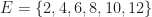$E= \{ 2,4,6,8,10,12 \}$ , or by implicitly stating the outcomes, e.g. we can also write $E=\{\text{ Even number }\}$ .)

For a given set of events, there may be more than one way to define the sample space of an experiment. E.g. if I want to know the sum of two dice, we could consider the set of outcomes for the first and second dice throw. (See table below)

Examples

Screenshot 2021-11-18 at 12.35.13

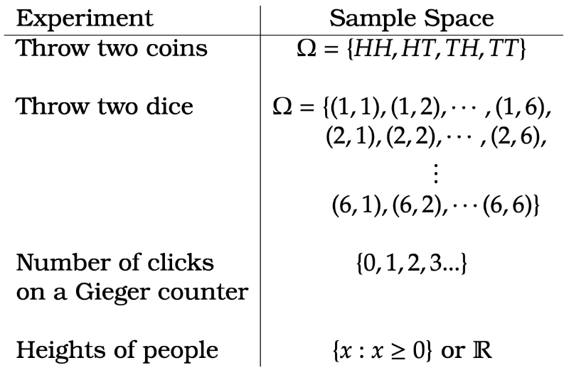
From the above table, note that sample spaces can be finite, (countably) infinite, or a continuum.

Definition of Discrete Probability.

For finite of countably infinite sample spaces, we can define probabilities as follows.

Definition [Probability – Discrete] For a sample space $\Omega= \{ \omega_1, \omega_2, \omega_3,... \}$ , probabilities are numbers $\mathbb P(\omega)$ for each $\omega \in \Omega$ such that

(Positive) For $\omega \in \Omega$ ,

$\mathbb P(\omega) \geq 0,$

(Sums to one)

$\sum_{\omega \in \Omega } \mathbb P(\omega ) = 1.$

For events, $E \subseteq \Omega$ , we get the probability of the event by summing

$\mathbb P (E ) = \sum_{\omega \in E } \mathbb P(\omega) \, .$

The above is a good definition of for finite (or countably infinite) sample spaces. When we consider probabilities for continuous sample spaces definitions need to be modified.

An informal definition. The above definition gives us a working mathematical definition for probability. That said it is worth noting that intuitively we consider probabilities to represent the long-run proportion of time an event (or outcome) has occurred in an experiment. So informally if we repeat a number of experiments, which we denote by #{experiment}, and for those we count the number of times an event occurs #{event $E$ occurs}, and if we let the number of experiments get large, that is $\# \{\text{experiment}\} \longrightarrow \infty$ , then it should hold that $\begin{aligned} \frac{\# \{\text{event $E$ occurs}\} }{ \# \{\text{experiment}\}} \longrightarrow \mathbb P( E)\, \label{probconv} %\end{aligned}$

Screenshot 2021-11-18 at 12.37.28

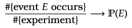
Later when we are a bit more precise about what we mean to “repeat a number of experiments”, the above statement will more formally be called the Law of Large Numbers.

Examples.

Example 1. For the experiment where we throw two coins, calculate

$\begin{aligned} \mathbb P( \text{at least one heads} ).\end{aligned}$

Answer 1. For the sample space $\Omega = \{ HH, HT, TH, TT\}$ , each probability is equally likely, i.e.

$\begin{aligned} p = \mathbb P( HH) = \mathbb P( HT) = \mathbb P( TH) = \mathbb P( TT) \, .\end{aligned}$

Also probabilities sum to one so

$\begin{aligned} 1 = \mathbb P( HH) + \mathbb P( HT) + \mathbb P( TH) + \mathbb P( TT) \end{aligned}$

This implies $4 p =1$ and so $p = \frac{1}{4}$ .

From this point there are two ways to solve the question:

Since $\;\{\text{at least one head}\}= \{ HH, HT, TH\}$ , we can directly sum over the outcomes in the event $\begin{aligned} \mathbb P( \text{at least one heads} ) =& \mathbb P( HH) + \mathbb P( HT) + \mathbb P( TH) \\ = & \frac{1}{4} + \frac{1}{4} + \frac{1}{4}\\ =& \frac{3}{4}\end{aligned}$
Since probabilities sum to one $\begin{aligned} 1 = \sum_{\omega \in \Omega} \mathbb P (\omega) = \mathbb P( \text{at least one heads} ) + \mathbb P( TT )\, ,\end{aligned}$ Thus $\begin{aligned} \mathbb P( \text{at least one heads} ) = 1- \mathbb P( TT ) = 1- \frac{1}{4} = \frac{3}{4}.\end{aligned}$

Example 2. A bag contains three green balls and a red ball. Two balls are taken out at random what is the probability that both are green?

Answer 2. Here are three ways to answer this question:

1. We can explicitly list by taking the balls out one at a time and count. Here we label the three green balls $G_1,G_2,G_3$ and the red ball $R$ . The probability space is $\begin{aligned} \Omega = \{ &\qquad\;\;\;\; (R,G_1),(R,G_2),(R,G_3)\\ & (G_1,R)\qquad\;\;\;\;,(G_1,G_2),(G_1,G_3)\\ & (G_2,R),(G_2,G_1)\qquad\;\;\;\;,(G_2,G_3)\\ & (G_3,R),(G_3,G_1),(G_3,G_2)\qquad\;\;\;\; \}\end{aligned}$ There are 12 equally likely outcomes and 6 outcomes with both green so $\begin{aligned} \mathbb P (\text{ both green } ) = \frac{6}{12} = \frac{1}{2}\, .\end{aligned}$ (Notice we had to label the three balls $G_1,G_2,G_3$ because if we did not, then $\mathbb P((G,R)) \neq \mathbb P( (R,G) )$ . So we could not count up events with equal probability.)
2. We can imagine we take out the balls simultaneously. Again we label the three green balls $G_1,G_2,G_3$ and the red ball $R$ . Recall we use curly brackets sets where the order does not matter, and we use round brackets when the order matters. (E.g. $(G_1,G_2) \neq (G_2,G_1)$ but $\{ G_1, G_2 \} = \{ G_2,G_1\}$ ). The probability space in this case is $\begin{aligned} \Omega = \{ & \{R,G_1\},\{R,G_2\},\{R,G_3\}\\ & \qquad\;\;\;\;,\{G_1,G_2\},\{G_1,G_3\}\\ & \qquad\qquad\qquad\;\;\;\;,\{G_2,G_3\} \}\end{aligned}$ There are 6 equally likely outcomes and 3 outcomes with both green so $\begin{aligned} \mathbb P (\text{ both green } ) = \frac{3}{6} = \frac{1}{2}\, .\end{aligned}$ 3. We can reason as follows. The probability the first ball removed is green is $3/4$ , as three out of four balls are green. Given the first ball is green, the probability the 2nd ball is green is $2/3$ , as now two out of three balls are green. So out of the three quarters of the time where the first ball is green, two thirds of the time the 2nd ball is green. Two thirds of three quarters is a half. So $\begin{aligned} \mathbb P (\text{ both green } ) = \frac{3}{4}\times \frac{2}{3} = \frac{1}{2} \, . \end{aligned}$ (This third argument might feel a little vague at first. We go into this in more detail when we discuss conditional probability, a bit later.)