(This is a section in the notes here.)
Counting in Probability. If each outcome is equally likely, i.e. 

 = \sum_{\omega \in \Omega } p= |\Omega | p") (where
(where 

 = \frac{1}{| \Omega |} \,\qquad \text{ for all } \omega \in \Omega .\end{aligned}")
Further, since 
 = \frac{\left|
E
\right|
}{|\Omega |} \, .\end{aligned}") So from the last two display equations above, we see that, when outcomes are equally likely, then to calculate probabilities we need to be able to count the number of outcomes in different sets.
So from the last two display equations above, we see that, when outcomes are equally likely, then to calculate probabilities we need to be able to count the number of outcomes in different sets.
Some Counting Rules. 1,2,3,4,… aside, we cover the following counting methods
- Multiplication
- Factorials
- Permutations
- Combinations
Card Game. We consider the probability of winning a card game in the following setting:
A card dealer has
cards
.
You are dealtcards.
You win if you get.
The probability of winning depends on what we mean by “the cards being dealt” and what is means by to “get A,K,Q”.
Multiplication.
Rules of the the card game. Suppose we play the card game in the following way
The dealer shuffles the deck. Shows a random card. Replaces it in the deck. And then repeats.
You win if you getthen
and then
, in that order.
The probability of winning. We can calculate the probability of winning as follows. The set of outcomes can be written as  : C_1,C_2,C_3 \in \{ A,K,Q,4,2\} \}\, .\end{aligned}") I.e. it is the set of triplets
I.e. it is the set of triplets 

 Since there is only one winning hand among these
 = \frac{1}{125}\,.
%\end{aligned}")

Note 


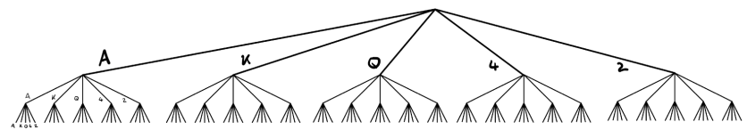
Figure 1. This card game has 5 possibilities at each stage.
In General. For sets 

 : \omega_1 \in \Omega_1,...,\omega_k \in \Omega_k) \big\}\,.
%\end{aligned}")

Following the argument as above we can see that 

For our card game, we had 

Factorials
Rules of the the card game. Suppose we play the card game in the following way
The dealer shuffles the deck. Shows a random card. Replaces it in the deck. And then repeats.
You win if you get
So now 

The probability of winning. Since the way that the dealer deals has not changed we know the probability of any hand, that is,  ) = \cdots = \mathbb P( ( Q,K,A) ) = \frac{1}{125}\, .
%\end{aligned}")

So if we want to calculate the probability of winning we need to calculate the number of events with a winning hand. It is not hard to check that , (A,Q,K), (K,A,Q), (K,Q,A),(Q,A,K),(Q,K,A) \}
%\end{aligned}")

That is there are 
 = \frac{6}{125}\, .
%\end{aligned}")

Six winning hands holds because.. Notice there are 


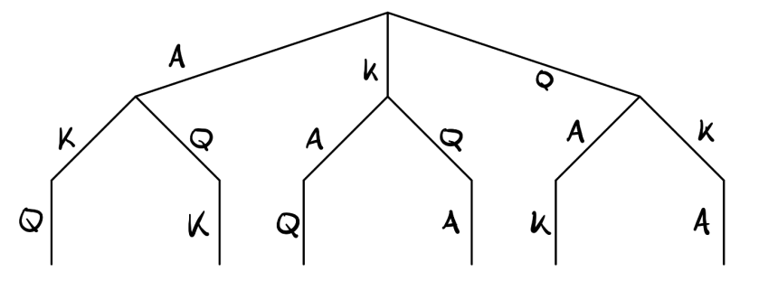
Figure 2. There are initially
In general. Given a set 

 : c_1,....,c_n \in C\text{ where }c_i \neq c_j\text{ for all } i \neq j \}
%\end{aligned}")

In general, following the argument as above it holds that  \times (n-2) \times .... \times 2 \times 1
%\end{aligned}")

Definition [Factorial] Given a positive integer 
 \times (n-2) \times .... \times 2 \times 1") (By convention we define
(By convention we define 
So 
Permutations
Rules of the the card game. Suppose we play the card game in the following way
The dealer shuffles the deck. Takes out a random card, but does to put it back in the deck . And then repeats.
You win if you get
The probability of winning. In this case, there is only one winning hand
 : C_1,C_2,C_3 \in \{ A,K,Q,4,2\} \text{ where } C_i \neq C_j \text{ for all } i \neq j \}\, .\end{aligned}")
As we will argue shortly 
 = \frac{1}{60}\, .
%\end{aligned}")

It holds that 


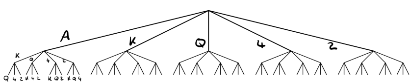
Figure 3. There are initially
In general. Given a set 
 : c_1,....,c_k \in C\text{ where }c_i \neq c_j\text{ for all } i \neq j \}
%\end{aligned}")

In general, following the argument as above it holds that  \times (n-2) \times .... \times (n-k+2) \times (n-k+1)
%\end{aligned}")
![]()
Definition [Permutation] Given non-negative integers 
 \times (n-2) \times .... \times (n-k+2) \times (n-k+1)") or more compactly using factorials:
or more compactly using factorials: !}")
So 
Combinations.
Rules of the the card game. Suppose we play the card game in the following way
The dealer shuffles the deck. Takes out a random card, but does not put it back in the deck . And then repeats.
You win if you get
The probability of winning. There are two ways to think about the above game. We focus first on the way that is most similar to out previous argument on permutations.
As before the ways of dealing the cards is exactly the same as our discussion on permutations.
 : C_1,C_2,C_3 \in \{ A,K,Q,4,2\} \text{ where } C_i \neq C_j \text{ for all } i \neq j \}\, .\end{aligned}") Thus
Thus 


 = \frac{3! \cdot 2!}{5!}=\frac{6}{60} = \frac{1}{10} \, .
%\end{aligned}")

A further way of thinking: removing the order… Rather than thinking of removing cards one at a time, we could think of taking out three cards at the same time from the deck of five cards, without paying attention to the order that they came out. Here we are interest in the set of three cards removed, e.g. 


We can think of this as dividing the deck of cards 
\qquad} \overset{|}{A}, \overset{\circ}{K}, \overset{|}{Q}, \overset{\circ}{4} ,\overset{|}{2}
& \rightarrow \{ \overset{|}{A}, \overset{|}{Q}, \overset{|}{2} \}\tag{cards dealt out}
\\&
\searrow \{ \overset{\circ}{K},\overset{\circ}{2} \} \tag{cards in the deck }
%\end{aligned}")
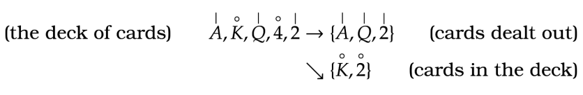
Here “

In addition to the above argument that gave in above. A way to think about counting the number of outcomes in 


There is only one outcome in  = \frac{1}{10}\,.
%\end{aligned}")

In General. Given a set 


In general the argument above gives that !}\,.
%\end{aligned}")

Definition [Combination] Given a non-negative integers 
!} \, .")
So 
Multinomials. In combinations the cards were dealt to one person (and the dealer) what if we wanted to consider dealing more hands. It is not hard to check that if there are 


Additional Remarks.
Here are a few additional remarks.
(These remarks are not examinable. So you may choose to skip, but it might yet be helpful).
A bit more interpretation for combinations. Notice earlier we thought of a combination as dividing up the deck of five cards:
 Here “

 (For this reason you can see that
Polynomials, Pascals Triangle. Consider the expansion of 
^n = {n \choose 0} + {n \choose 1} x + {n \choose 2} x^2 + ...+ {n \choose n} x^n \, .
%\end{aligned}")

Why? Well for instance if we look at the 


 (\overset{\circ}{1}+x) ( 1+\overset{|}{x}) ( \overset{\circ}{1}+ x) (1+\overset{|}{x}) \, .\end{aligned}") This is the same as
This is the same as 

The Binomial Theorem. Notice from the above result we can see that 

Hint: 
Pascal’s Triangle. If we repeatedly apply the above formula we get a nice shape for listing out combinations:  This is called Pascal’s Triangle.
Stirlings Formula. When } e^{-n} n^n") Here the
Here the 
Examples
Example. What is the probability of winning the jackpot in the national lottery (lotto)?
(Recall the national lottery 
Answer. The number of draws in 

Example. What is the probability of winning the jackpot in Euromillions?
(Recall that Euromillions has 

Answer. The total number of combinations for the main numbers is 


Example. How many distinct words can be made out of 
Answer. 

Example. How many distinct words can be made out of 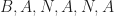
Answer. 
Example [Birthday Paradox] In a football game there are 23 players (including the referee). What is the probability that two or more players have the same birthday.1
Answer. Note that 
= 1 - \mathbb P ( \text{all different} ) \, .
%\end{aligned}")

So we need to count the number of ways the birthdays can be organized and the number of ways that all birthdays can be different. Notice that the sample space has size ^{23} \, .") (I.e. Notice that the number of birthday for the 1st player is 365, and for the 2nd player it is 365 and so forth), whereas the number of ways the players can have different birthdays is a permutation:
(I.e. Notice that the number of birthday for the 1st player is 365, and for the 2nd player it is 365 and so forth), whereas the number of ways the players can have different birthdays is a permutation: 

(I.e. Notice that the number of birthday for the 1st player is 365, and for the 2nd player it is 364 – because player
Thus  = \frac{P_{23}^{365}}{365^{23}}
= 0.4927
%\end{aligned}")

and  = 0.5073 \, .
%\end{aligned}")
![]()
The result may be quite surprising as you would think it unlikely to share a birthday with any individual. However, there are many pairs of birthdays between the players. These balance out to give 50% chance of two players having the same birthday.
Example. A parking inspector randomly inspects 

Answer. The number of ways of inspecting 


We can suppose, without loss of generality, that the first 

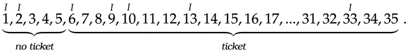
Here “


Thus  = \frac{{ 5 \choose 2} \times { 30 \choose 5}}{{35 \choose 7}}
= 0.212 \, .
%\end{aligned}")

- You can ignore Feb 29th on leap years.↩
