Discrete Probability Distributions

There are some probability distributions that occur frequently. This is because they either have a particularly natural or simple construction. Or they arise as the limit of some simpler distribution. Here we cover

Bernoulli random variables
Binomial distribution
Geometric distribution
Poisson distribution.

(This is a section in the notes here.)

Of course there are many other important distributions. Like with counting, it is often easy when first learning about probability to think of different probability distributions as being a main destination for probability. However, it is perhaps better to think of the probability distributions that we cover now as simple building blocks that we can then be later used to construct more expressive probabilistic and statistical models.

Again we focus on probability distributions that take discrete values though shortly we will begin to discuss their continuous counterpart.

Notation. There are many different distributions which often have different parameters. For instance, shortly we will define the Binomial Distribution, which has two parameters $n$ and $p$ and we denote by $\text{Bin}(n,p)$ . If a random variable $X$ has a specific distribution then we use “ $\sim$ ” to denote this. E.g. if $X$ is a random variable with parameters $n=4$ and $p=0.2$ then we write $\begin{aligned} X \sim \text{Bin}(4,0.2) \, . %\end{aligned}$

Screenshot 2021-11-18 at 15.53.30

Bernoulli Distribution.

We start with the simplest discrete probability distribution.

Definition [Bernoulli Distribution] A random variable that is either zero or one is a Bernoulli random variable. That is we we write $X \sim \text{Bern}(p)$ if

$\begin{aligned} \mathbb P(X=1) = p \qquad \text{and} \qquad \mathbb P(X=0) =1-p \,.\end{aligned}$

It is a straight-forward calculation to show that

Screenshot 2021-11-18 at 15.54.34

for $X \sim \text{Bern}(p)$ $\begin{aligned} \mathbb E [ X] = p , \qquad \text{and} \qquad \mathbb V(X) = p(1-p) \,. %\end{aligned}$

Binomial Distribution.

If we take $X_1,X_2,...,X_n$ to be independent Bernoulli random variables with parameter $p$ , and we add then together $\begin{aligned} X = \sum_{i=1}^n X_i \,, %\end{aligned}$

Screenshot 2021-11-18 at 15.55.25

then we get a Binomial distribution with parameters $n$ and $p$ .

So if we consider an experiment with probability of success $p$ and we repeat an experiment $n$ times and count up the number of successes, then the resulting probability distribution is a Binomial distribution.

Let’s briefly consider the probability that $X=k$ . One event where $\{ X=k \}$ occurs is when the first $k$ experiments end in success and the rest fail, $\{X_1=1, ..., X_k=1, X_{k+1} = 0 ,..., X_n = 0 \}$ . Note that by independence $\begin{aligned} & \mathbb P (X_1=1, ..., X_k=1, X_{k+1} = 0 ,..., X_n = 0 ) \\ &= \mathbb P (X_1=1) ... \mathbb P( X_k=1) \mathbb P( X_{k+1} = 0 ) ... \mathbb P( X_n = 0 ) \notag \\ & = p^k (1-p)^{n-k} %\end{aligned}$

Screenshot 2021-11-18 at 15.56.14

Indeed the probability of any individual sequence $X_1,...,X_n$ where $\sum_i X_i = k$ . So how may such sequences are there? Well we have seen this before. It is the number of ways we can label $n$ points with $k$ ones (see additional remarks on combinations in Section [sec:Counting]), that is the combination $C^n_k$ . Thus we have $\begin{aligned} \mathbb P (X = k ) = { n \choose k} p^k (1-p)^{n-k} \, . %\end{aligned}$

Screenshot 2021-11-18 at 15.56.47

This motivates the following definition.

Definition [Binomial Distribution] A random variable $X$ has a binomial distribution with parameters $n$ and $p$ , if it has probability mass function $\begin{aligned} p(k ) = { n \choose k} p^k (1-p)^{n-k} \, , %\end{aligned}$

Screenshot 2021-11-18 at 15.57.13

for $k=0,1,...n$ , and we write $X \sim \text{Bin}(n,p)$ .

Here are some results on Binomial distributions that might be handy.

Lemma 1. If $X \sim \text{Bin}(n,p)$ , then $\begin{aligned} \mathbb E[X] =np , \quad \text{and} \quad \mathbb V(X) = n p (1-p) \, . %\end{aligned}$

Screenshot 2021-11-18 at 15.59.10

Lemma 2. If $X \sim \text{Bin}(n,p)$ and $Y \sim \text{Bin}(m,p)$ and are independent then $\begin{aligned} X+Y \sim \text{Bin} ( n+m ,p) \, . %\end{aligned}$

Proof. $X= \sum_{i=1}^n X_i$ for $X_i$ independent and $X_i \sim \text{Bern}(p)$ , and $X= \sum_{i=n+1}^m X_i$ for $X_i$ independent and $X_i \sim \text{Bern}(p)$ . So $X+Y = \sum_{i=1}^{n+m} X_i$ thus is Bernoulli with parameters $n+m$ and $p$ .

Lemma 3. If $X \sim Bin(n,p)$ and $Y_1,...,Y_n$ are independent Bernoulli random variables with parameter $q$ then $\begin{aligned} \sum_{i=1}^X Y_i \sim Bin ( n,pq) \, . %\end{aligned}$

Screenshot 2021-11-18 at 16.01.00

Proof. Since we can write $X= \sum_{i=1}^n X_i$ for $X_i \sim \text{Bern}(p)$ . Note that an equivalent way to represent the above random variable is $\begin{aligned} \sum_{i=1}^n X_i Y_i \end{aligned}$ Since $X_i Y_i \sim \text{Bern}(pq)$ , then the above random variable must be $\text{Bin}(n,pq)$ . $\square$

Geometric Distribution

Suppose we throw a biased coin until the first time that it lands on heads. The distribution of the number of throws is a geometric distribution. For instance, the probability that it takes $X=5$ coin throws is the same as the probability of $4$ tails in a row and then one heads which is $\begin{aligned} \mathbb P (X = 5) = \mathbb P( TTTTH) = (1-p)^4 p %\end{aligned}$

Screenshot 2021-11-18 at 16.01.57

where $p$ is the probability of heads. In general, the probability we need $k$ throws is $\begin{aligned} \mathbb P( X=k) = (1-p)^k p \, . %\end{aligned}$ Screenshot 2021-11-18 at 16.02.00

This gives the geometric distribution.

Definition [Geometric distribution] The geometric distribution with success probability $p$ is the distribution with probability mass function $\begin{aligned} p(k ) = (1-p)^{k-1} p %\end{aligned}$

Screenshot 2021-11-18 at 16.03.03

for $k=1,2,...$ , and we write $X \sim \text{Geo}(p)$ .

The following lemma is useful for geometrics distributions but also various forms of compound interest and other applications.

Lemma 4. [Geometric Series]For $|x| <1$ ,

$\begin{aligned} \sum_{n=0}^\infty x^n = \frac{1}{1-x},\quad \sum_{n=0}^\infty n x^{n-1} = \frac{1}{(1-x)^2} \quad \text{and} \quad \sum_{n=0}^\infty n(n-1) x^{n-2} =\frac{2}{(1-x)^3}\end{aligned}$

Proof.

$\begin{aligned} \sum_{n=0}^\infty x^n = 1+ &x+ x^2 +x^3+ ... \notag \\ x \times \sum_{n=0}^\infty x^n =\quad\; & x+x^2+x^3 + ...\end{aligned}$

Now subtracting gives $\begin{aligned} (1-x)\sum_{n=0}^\infty x^n = 1 %\end{aligned}$

Screenshot 2021-11-18 at 16.04.37

Thus

$\begin{aligned} \sum_{n=0}^\infty x^n = \frac{1}{ (1-x)} \,.\end{aligned}$

Differentiating the above with respect to $x$ gives

$\begin{aligned} \sum_{n=0}^\infty n x^{n-1}=\sum_{n=0}^\infty \frac{d}{dx}x^n=\frac{d}{dx}\sum_{n=0}^\infty x^n = \frac{d}{dx}\frac{1}{ (1-x)} = \frac{1}{(1-x)^2} \,.\end{aligned}$

Differentiating again gives

$\begin{aligned} \sum_{n=0}^\infty n(n-1) x^{n-2} =\frac{2}{(1-x)^3} \, .\end{aligned}$

$\square$

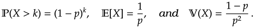
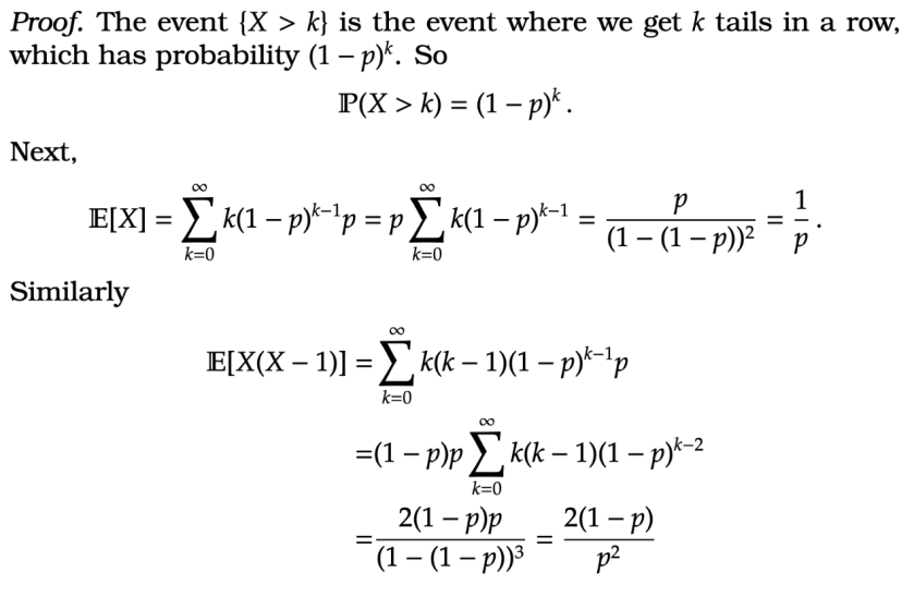
Lemma 4. If $X \sim \text{Geo}(p)$ then $\begin{aligned} \mathbb P (X > k) = (1-p)^k, \quad \mathbb E[ X] = \frac{1}{p} ,\quad \text{and} \quad \mathbb V(X) = \frac{1-p}{p^2} \, . %\end{aligned}$

Screenshot 2021-11-18 at 16.05.54

Screenshot 2021-11-18 at 16.06.54

Screenshot 2021-11-18 at 16.07.35

If we throw a coin and get $8$ tails in a row, and we ask how long should we wait until we next get a heads, then (even though it might feel like we are now due a heads) it is the same as the time we would have expected when we first started throwing the coin. This is key property of the geometric distribution and its called memoryless property.

Lemma 5. [Memoryless Property] If $T \sim Geo(p)$ then, conditional on $\{ T > t \}$ , the distribution of $T-t$ is geometrically distributed with parameter $p$ . In otherwords $(T-t | T \geq t) \sim Geo(p)$ .

Proof.

$\begin{aligned} \mathbb P ( T-t > k | T >t ) = & \frac{\mathbb P(T > t+k , T> t) }{\mathbb P(T >t)} \notag \\ = & \frac{\mathbb P(T > t+k)}{\mathbb P(T>t)} \notag \\ = & \frac{(1-p)^{t+k}}{(1-p)^t} = (1-p)^k\end{aligned}$

$\square$

Example [Waiting for a bus] At a bus stop, the probability that a bus arrives at any given minute is $p$ and is independent from one minute to the next.

What is the expect gap in the time between any two busses?
You arrive at the bus stop and there is no bus there. What is the expected gap between the last time a bus arrived and the next bus to arrive?

Answer. 1. The time from one bus to the next is geometric $p$ , so the expected wait is $1/p$ .

2. Given you at a time with no bus the time until the last bus too arrive is geometrically distributed with parameter $p$ and so is the time until the next bus to arrive. The time between this bus arrivals is thus the sum of these geometeric distributions, and so the expected time is $2/p$ .

This is sometimes called the waiting time paradox. Here we see that when we turn up at the bus station the gap between the buses is twice as long as the mean time between the buses. This is because when we turn up and there is no bus there then we are more likely to have chosen a time with a bigger gap between the buses.

Poisson Distribution.

The Poisson distribution arises when we count the number of successes of an unlikely event over a large population. This occurs in all manner of settings from nuclear decay, to insurance, to call over a telephone line.

We present a definition first and then we will motivate the Poisson distribution.

Definition [Poisson distribution] For a parameter $\lambda >0$ , the Poisson distribution has probability mass function $\begin{aligned} p(k) = \frac{\lambda^k}{k!} e^{\lambda} %\end{aligned}$

Screenshot 2021-11-18 at 16.09.26

for $k=0,1,2,...\,$ and we write $X \sim Po(\lambda)$

Motivation for Poisson Distribution. If we take a Binomial distribution where the number of trails $n$ is large but the probability of success in each trail is small, specifically $p=\lambda /n$ , then the Binomial distribution is well approximated by a Poisson distribution.

This is the reason the Poisson distribution is a reasonable distribution to represent pheonomena like nuclear decay. In nuclear decay, there are a large number of atoms in a radio-active substance, and, in any given time interval, there is a very small probability of one of these atom undergoing nuclear decay and the emitting a particle (e.g. a gamma-ray). For this reason the distribution of the number of observed gamma-rays over a time interval is well approximated by a Poisson distribution.

The following lemma sets out how the Poisson distribution approximates the Binomial distribution (again students primarily interested in assessment can skip with argument).

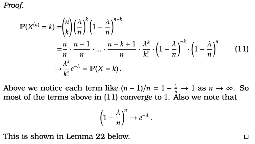
Theorem 1 [Binomial to Poisson Limit] Consider a sequence of Binomial random variables 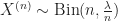$X^{(n)} \sim \text{Bin}(n , \frac{\lambda}{n} )$ for $n \in \mathbb N$ , and let $X \sim Po(\lambda)$ . Then $\begin{aligned} \mathbb P(X^{(n)} = k ) \xrightarrow[n \rightarrow \infty]{} \mathbb P(X =k) %\end{aligned}$

Screenshot 2021-11-18 at 16.10.20

That is as $n$ gets large the probability of $X^{(n)}=k$ approaches the probability that $X=k$ for each $k$ . $\begin{aligned} \mathbb P (X^{(n)} = k ) =& { n \choose k} \left( \frac{\lambda}{n} \right)^k \left( 1- \frac{\lambda}{n} \right)^{n-k} \notag \\ = & \frac{n}{n} \cdot \frac{n-1}{n} \cdot... \cdot\frac{n-k+1}{n} \cdot \frac{\lambda^k}{k!} \cdot \left( 1- \frac{\lambda}{n} \right)^{-k} \cdot \left( 1- \frac{\lambda}{n} \right)^n \label{PoLongEquation} \\ \rightarrow & \frac{\lambda^k}{k!} e^{-\lambda} = \mathbb P(X=k) \,. \notag %\end{aligned}$ Screenshot 2021-11-18 at 16.11.14

Screenshot 2021-11-18 at 16.11.25

Now for some more standard facts about the Poisson distribution.

Screenshot 2021-11-18 at 16.12.38

Lemma 6 [Poisson Summation Property] If $X \sim Po(\lambda)$ , $Y \sim Po (\mu)$ , and $X$ and $Y$ are independent then $X + Y \sim Po(\lambda+ \mu).$

Lemma 7 [Poisson Thinning Property] If $N \sim Po(\lambda)$ and, independent of $N$ , we let $X_1,X_2,...$ be independent Bernoulli random variables with parameter $p$ then $\begin{aligned} \sum_{n=1}^N X_i \sim Po (p\lambda )\, . %\end{aligned}$

In Lemma 6, we can begin to see how we can think of a Poisson distribution as part of a process that evolves in time. For instance we might say that the number of calls on a set of telephone lines in each minute is Poisson distributed with mean $4$ , then the number of calls per hour is Poisson mean $4\times 60 = 240$ .

In Lemma 7, we can see that if we exclude points according to an independent random variable then the resulting random variable is still Poisson. This is useful for instance in insurance. Here the number of claims an insurance company receives in a given day might be Poisson with mean $20$ . The company might split the claims into big and small claims (say on average half the claims are big and half small). Since there is some fixed probability that each claim is, say, big then the resulting number of big claims is Poisson mean $10$ . This is useful for an insurance company as they can divide up, reinsure or resell some of their risk.

Both lemmas can be proved directly by summing things but is a bit of a messy calculation. Intuitively the above lemmas holds because an equivalent results, Lemma 2 and Lemma 3, hold for Binomial random variables. So the both properties persists when we take the limit to a Poisson random variable (like in Theorem 1). The cleanest proof (using moment generating functions) is beyond the scope of this course, so we omit the proof for now.

Bernoulli Distribution.

Binomial Distribution.

Geometric Distribution

Poisson Distribution.

Share this:

Like this:

Leave a Reply Cancel reply