Markov Decision Processes

Markov decision processes are essentially the randomized equivalent of a dynamic program.

A Random Example

Let’s first consider how to randomize the tree example introduced.

Below is a tree with a root node and four leaf nodes colored grey. At the route node you choose to go left or right. This incurs costs $4$ and $2$ , respectively. Further, after making this decision there is a probability for reaching a leaf node. Namely, after going left the probabilities are $0.5$ & $0.75$ , and for turning right, the probabilities are $0.25$ & $0.75$ . For each leaf node there is there is a cost, namely, $2, 3, 6,$ and $1$ .

Screenshot 2019-01-26 at 10.34.56.png

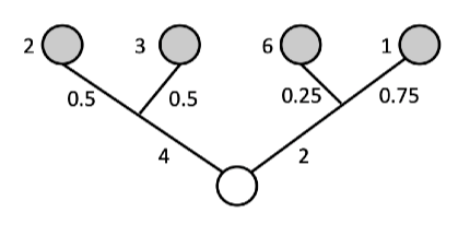
Given you only know the probabilities (and not what happens when you choose left or right), you’d want to take the decision with lowest expected cost. The expected cost for left is $4+ 0.5 \times 2 + 0.3 \times 3 = 5.5$ and for right is $2+ 0.25 \times 6 + 0.75 \times 1 = 4.25$ . So go right.

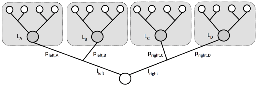
Below we now replace the numbers above with symbols. At the route node you can choose the action to go left or right. These, respective, decisions incur costs of $l_{\text{left}}$ and $l_{\text{right}}$ . After choosing left, you will move to state $A$ with probability $p_{\text{left},A}$ or to state $B$ with probability $p_{\text{left},B}$ and similarly choosing right states $C$ & $D$ can be reached with probabilities $p_{\text{left},C}$ & $p_{\text{left},D}$ . After reaching node $A$ (resp. $B$ , $C$ , $D$ ) the total expected cost thereafter is $L_A$ (resp. $L_B$ , $L_C$ , $L_D$ ).

Screenshot 2019-01-26 at 10.36.40.png

Show that the optimal expected cost from the route node, $L_R$ satisfies

$L_R = \min_{a\in \{ \text{left}, \text{right}\} } \left\{ l_a + {\mathbb E}_a \left[ L_{X_a}\right]\right\}.$

where here the random variable $X_a$ denotes the state in $\{A,B,C,D\}$ reached after action is taken. The cost from choosing “left“ is :

$l_{\text{left}} + p_{\text{left},A} L_{A} + p_{\text{left},B} L_{B} = l_{\text{left}} + \mathbb E_{\text{left}} [L_{\text{left}}]$

and the cost for choosing “right” is:

$l_{\text{right}} + p_{\text{right},A} L_{A} + p_{\text{right},B} L_{B} = l_{\text{right}} + \mathbb E_{\text{right}} [L_{\text{right}}].$

The optimal cost is the minimum of these two is

$L_R = \min_{a\in \{ \text{left}, \text{right}\} } \left\{ l_a + {\mathbb E}_a \left[ L_{X_a}\right]\right\}.$

where here the random variable $X_a$ denotes the state in $\{A,B,C,D\}$ reached after action is taken. Notice how we abstracted away the future behaviour after arriving at $A$ , $B$ , $C$ , $D$ . Into a single cost for each state: $L_A$ , $L_B$ , $L_C$ , $L_D$ . And we can propagate this back to get the costs at the route state $R$ . I.e. we can essentially apply the same principle as dynamic programming here.

Definitions

A Markov Decision Process (MDP) is a Dynamic Program where the state evolves in a random (Markovian) way.

Def [Markov Decision Process] Like with a dynamic program, we consider discrete times $t=0,1,...,T$ , states $x\in\mathcal{X}$ , actions $a\in\mathcal{A}_t$ and rewards $r_t(a,x)$ . However, the plant equation and definition of a policy are slightly different.

Like with a Markov chain, the state evolves as a random function of the current state and action, $f: \mathcal{X}\times \mathcal{A}_t \times [0,1] \rightarrow \mathcal{X}$ . Here

$X_{t+1} = f(X_t,a_t; U_t) \equiv f(X_t,a_t)$

where $(U_t)_{t\geq 0}$ are IIDRVs uniform on $[0,1]$ . This is called the Plant Equation.

A policy $\pi$ choses an action $\pi_t$ at each time $t$ as a function of past states $x_0,...,x_t$ and past actions $\pi_0,...,\pi_{t-1}$ . We let $\mathcal{P}$ be the set of policies. A policy, a plant equation, and the resulting sequence of states and rewards describe a Markov Decision Process.

As noted in the equivalence above, we will usually suppress dependence on $U_t$ . Also, we will use the notation

$\mathbb{E}_{x_t, a_t} [G({X}_{t+1})] = \mathbb{E} [G(F_t(x_t,a_t;U))] \quad\text{and} \quad \mathbb{E}_{x, a} [G(\hat{X})] = \mathbb E [ G(f(x,a;U))]$

where here and here after we use $\hat{X}$ to denote the next state (after taking action $a$ in state $x$ ). Notice in both equalities above, the term on the right depends on only one random variable, $U$ .

Objective is to find a process that optimizes the expected reward.

Def [Markov Decision Problem] Given initial state $x_0$ , a Markov Decision Problem is the following optimization Screenshot 2019-01-26 at 10.42.01.png Further, let $R_\tau({x_\tau, \Pi})$ (Resp. $V_\tau(x_\tau)$ ) be the objective (Resp. optimal objective) for when the summation is started from time $t=\tau$ and state $X_\tau=x_\tau$ , rather than $t=0$ and $X_0=x_0$ . We often call $V$ to value function of the MDP.

The next result shows that the Bellman equation follows essentially as before but now we have to take account for the expected value of the next state.

Def [Bellman Equation] Setting $V_T(x)=r_T(x)$ for $t=T-1,T-2,...,0$

$\tag{Bell eq.} V_t(x_t) = \max_{a_t\in\mathcal{A}_t} \left\{ r_t(x_t,a_t) + \mathbb{E}_{x_t,a_t} \left[ V_{t+1}(X_{t+1})\right] \right\}.$

The above equation is Bellman’s equation for a Markov Decision Process.

Let $\mathcal{P}_t$ be the set policies that can be implemented from time $t$ to $T$ . Notice it is the product actions at time $t$ and the set of policies from time $t+1$ onward. That is $\mathcal{P}_t = \{ (\pi_t,\Pi): \Pi \in\mathcal{P}_{t+1}, \pi_t: \mathcal{X}^t \times \prod_{\tau = 0}^{t-1}\mathcal{A}_\tau \rightarrow \mathcal{A}_t \}$ .

$\begin{aligned} V_t(x_t) &= \max_{\Pi_t \in \mathcal{P}_t} \mathbb{E}_{x_t \pi_t} \left[ \sum_{t=0}^{T-1} r_t(X_t,\pi_t) + r_T(X_T) \right]\\ &= \max_{\pi_t } \max_{\Pi \in \mathcal{P}_{t+1}} \Bigg\{ r_t(x_t,\pi_t) + \mathbb{E}_{x_t \pi_t} \Bigg[ \mathbb{E}_{X_{t+1} \pi_{t+1}} \Bigg[ \sum_{\tau=t+1}^{T-1} r_{\tau}(X_\tau,\pi_\tau) + r_T(X_T) \Bigg]\Bigg]\Bigg\}\\ &= \max_{a\in\mathcal{A} } \Bigg\{ r_t(x_t,a) + \mathbb{E}_{x_t\, a} \Bigg[ \underbrace{ \max_{\Pi \in \mathcal{P}_{t+1}} \mathbb{E}_{X_{t+1} \pi_{t+1}} \Bigg[ \sum_{\tau=t+1}^{T-1} r_{\tau}(X_\tau,\pi_\tau) + r_T(X_T) \Bigg] }_{ =V_{t+1}(x_{t+1}) } \Bigg]\Bigg\} \end{aligned}$ 2nd equality uses structure of $\mathcal{P}_t$ , takes the $r_t$ term out and then takes conditional expectations. 3rd equality takes the supremum over $\mathcal{P}_{t+1}$ , which does not depend on $\pi_t$ , inside the expectation and notes the supremum over $\pi_t$ is optimized at a fixed action $a\in\mathcal{A}$ (i.e. the past information did not help us.)

Ex. You need to sell a car. At every time $t=0,...,T-1$ , you set a price $p_t$ and a customer then views the car. The probability that the customer buys a car at price $p$ is $D(p)$ . If the car isn’t sold be time $T$ then it is sold for fixed price $V_T$ , $V_T<1$ . Maximize the reward from selling the car and find the recursion for the optimal reward when $D(p) = (1-p)_+$ .

Ex. You own a call option with strike price $p$ . Here you can buy a share at price $p$ making profit $X_t-p$ where $x_t$ is the price of the share at time $t$ . The share must be exercised by time $T$ . The price of stock $X_t$ satisfies $X_{t+1} = X_t + \epsilon_t$ for $\epsilon_t$ IIDRV with finite expectation. Show that there exists a decresing sequence $\{a_t\}_{0\leq t \leq T}$ such that it is optimal to exercise whenever $X_s \geq a_s$ occurs.

Ex. You own an expensive fish. Each day you are offered a price for the fish according to a distribution density $f(x)$ . You make the accept or reject this offer. With probability $1-p$ the fish dies that day. Find the policy that maximizes the profit from selling fish.

Ex. Consider an MDP where rewards are now random, i.e. after we have specified the state and action the reward $r(x,a)$ is still an independent random variable. Argue that this is the same as a MDP with non-random rewards given by $\bar{r}(x,a) = \mathbb E [r(x,a)]$

Ex. Indiana Jones is trapped in a room in a temple. There are $n$ passages that he can try and escape from. If he attempts to escape from passage $i\in \{1,...,n\}$ then either: he esacapes with probability $p_p$ ; he dies with probability $q_i$ ; or with probability $r_i=1-p_i-q_i$ the passage is a deadend and he returns to the room which he started from. Determine the order of passages which Indiana Jones must try in order to maximize his probability of escape.

Ex. You invest in properties. The total value of these properties is $x_t$ in year $t=1,...,T$ .
Each year $t$ , you gain rent of $rx_t$ and you choose to consume a proportion $a_t\in [0,1]$ of this rent. The remaining proportion is reinvested in buying new property.
Further you pay mortgage payments of $m x_t$ which are deducted from your consumed wealth. Here $m<r$ .
Your objective is to maximize the wealth consumed over $T$ years.

Briefly explaining why we can express this problem as a finite time dynamic program with
$f(x,a)=x + rx(1-a),\qquad r_t(x,a) = x(ra-m),\qquad r_T(x)=0\ ,$
prove that if $W_{T-s}(x) = x \rho_{s}$ for some constant $\rho_s$ then
$\rho_s = \max \{ r - m +\rho_{s-1}, (1+r)\rho_{s-1} -m \} .$