Dynamic Programming

We briefly explain the principles behind dynamic programming and then give its definition.

An Introductory Example

In the figure below there is a tree consisting of a root node labelled $R$ and two leaf nodes colored grey. For each edge, there is a cost. Your task is to find the lowest cost path from the root node to a leaf.

There are a number of ways to solve this, such as enumerating all paths. However, we are interested in one approach where the problem is solved backwards, through a sequence of smaller sub-problems. Specifically, once we reach the penultimate node on the left (in the dashed box) then it is clearly optimal to go left with a cost of $1$ . This solves an easier sub problem and, after solving each sub problem, we can then attack a slightly bigger problem. If we solve for each leaf in this way we can solve the problem for the antepenultimate nodes (the node before the penultimate node).

Thus the problem of optimizing the cost of the original tree can be broken down to a sequence of much simpler optimizations given by the shaded boxed below.

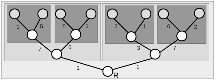
From this we see the optimal path has a cost of $5$ and consists of going right, then left, then right.

Let’s consider the problem a little more generally in the next figure. The tree on the righthand-side has a lowest cost path of value $L_{rhs}$ and the lefthand-side tree has lowest cost $L_{lhs}$ and the edges leading to each, respective tree, have costs $l_{rhs}$ and $l_{lhs}$ . Once the decision to go left or right is made (at cost $l_{rhs}$ or $l_{lhs}$ ) it is optimal to follow the lowest cost path (at cost $L_{rhs}$ or $L_{lhs}$ ). So $L$ , the minimal cost path from the root to a leaf node satisfies

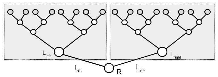
Similarly, convince yourself that the same argument applies from any node $x$ in the tree network that is

$L_x = \min_{a \in \{ lhs, rhs \}} \left\{ l_{a} + L_{x(a)} \right\}.$

where $L_{x}$ is the minimum cost from $x$ to a leaf node and where for $a\in\{lhs,rhs \}$ $x(a)$ is the node to the lefthand-side or righthand-side of $x$ . The equation above is an example of the Bellman equation for this problem, and in our example, we solved this equation recursively starting from leaf nodes and working our way back to the root node.

The idea of solving a problem from back to front and the idea of iterating on the above equation to solve an optimisation problem lies at the heart of dynamic programming.

Definition

We now give a general definition of a dynamic programming:

Time is discrete $t=0,1,...,T$ ; $x_t\in \mathcal{X}$ is the state at time $t$ ; $a_t\in \mathcal{A}_t$ is the action at time $t$ ; The state evolves according to functions $f_t: \mathcal{X}\times \mathcal{A}_t \rightarrow \mathcal{X}$ . Here

$x_{t+1}= f(x_t, a_t). \label{DP:Plant}\tag{Plant eq}$

This is called the Plant Equation. A policy $\pi$ choses an action $\pi_t$ at each time $t$ . The (instantaneous) reward for taking action $a$ in state $x$ at time $t$ is $r_t(a,x)$ and $r_T(x)$ is the reward for terminating in state $x$ at time $T$ .

Def.[Dynamic Program] Given initial state $x_0$ , a dynamic program is the optimization Screenshot 2019-01-26 at 10.20.12.png

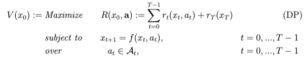
Further, let $R_\tau(x_{\tau},{\bf a})$ (Resp. $V_\tau(x_\tau)$ ) be the objective (Resp. optimal objective) for when the summation is started from $t=\tau$ , rather than $t=0$ .

Thrm [Bellman’s Equation] $V_T(x) = r_T(x)$ and for $t=T-1,...,0$

where $x_t\in\mathcal{X}$ and $x_{t+1}=f_t(x_t,a_t)$ .

Proof. Let ${\bf a}_t=(a_t,...,a_{T-1})$ . Note that $R_{t}(x_{t},{\mathbf a}_t) = r_t(x_t,a_t) + R_{t+1}(x_{t+1},{\mathbf a}_{t+1}).$

$\begin{aligned} V_t(x_t) &= \max_{{\bf a}_t} \left\{ R_t(x_t,{\bf a}_t) \right\} = \max_{a_t} \max_{{\bf a}_{t+1}}\left\{ r_{t}(x_t,a_t) + R_{t+1}({x_{t+1},\bf a}_t) \right\} \\ &= \max_{a_t} \left\{ r_{t}(x_t,a_t) +\max_{{\bf a}_{t+1}} R_{t+1}(x_{t+1},{\bf a}_t) \right\} =\max_{a_t\in\mathcal{A}_t}\left\{ r_t(x_t,a_t) + V_{t+1} (x_{t+1}) \right\} . \end{aligned}$