Infinite Time Horizon

Thus far we have considered finite time Markov decision processes. We now want to solve MDPs of the form $V(x) = \maxi_{\Pi \in {\mathcal P} } \quad R(x,\Pi) := \mathbb{E}_{x_0} \left[ \sum_{t=0}^{\infty} \beta^{t} r(X_t,\pi_t) \right] \, .$

We can generalize Bellman’s equation to infinite time, a correct guess at the form of the equation would, for instance, be

$V(x) = \max_{a\in {\mathcal A}} \Big\{ r(x,a) + \beta {\mathbb E}_{x,a} \left[ V(\hat{X}) \right] \Big\}, \qquad x\in \mathcal X\, .$

Previously we solved Markov Decisions Processes inductively with Bellman’s equation. In infinite time, we can not directly apply induction; however, we see that Bellman’s equation still holds and we can use this to solve our MDP. For now we will focus on the case of discounted programming: here we assume that

$\max_{x\in \mathcal X, a\in \mathcal A} |r(x,a) | < \infty \qquad \text{and} \qquad \beta \in (0,1)\, .$

We will cover cases where $\beta=1$ later.

At this point it is useful define the concept of a $Q$ -factor. A Q-factor of a policy $\pi$ is the reward that arises when we take action $a$ from state $x$ and then follow policy $\pi$ .

Def. [Q-Factor] The $Q$ -factor of reward function $R(\cdot)$ is the value for taking action $a$ in state $x$

$Q_R(x,a) = \mathbb E_{x,a} [ r(x,a) + \beta R(\hat{X}))]\, .$

Similarly the $Q$ -factor for a policy $\pi$ , denoted by $Q_{\pi}(x,a)$ , is given by the above expression with $R(x) = R(x,\pi)$ . The Q-factor of the optimal policy is given by

$Q^*(x,a) =\max_{\pi} Q_{\pi}(x,a).$

The following result shows that if we have solved the Bellman equation then the solution and its associated policy is optimal.

Thrm. For a discounted program, the optimal policy $V(x)$ satisfies

$V(x) = \max_{a\in {\mathcal A}} \Big\{ r(x,a) + \beta {\mathbb E}_{x,a} \left[ V(\hat{X}) \right] \Big\}.$

Moreover, if we find a function $R(x)$ such that

$R(x) = \max_{a\in {\mathcal A} } \left\{ r(x,a) + \beta \mathbb{E}_{x,a} \left[ R(\hat{X}) \right] \right\}$

then $R(x) = V(x)$ , i.e. the solution to the Bellman equation is unique, and we find a function $\pi(x)$ such that

$\pi(x) \in \argmax_{a\in \mathcal A} \left\{ r(x,a) + \beta \mathbb E_{x,a} \left[ R(\hat{X}) \right] \right\}$

Then $\pi$ is optimal and $R(x,\pi)=R(x)=V(x)$ the optimal value function.

Proof. We know that $R_t(x,\Pi) = r(x,\pi_0) + \beta \mathbb E [ R_{t-1}(\hat{X},\hat{ \Pi} ) ].$ Applying limits as $t\rightarrow \infty$ on both sides and bounded convergence theorem gives that

$\begin{aligned} R(x,\Pi) & = r(x,\pi_0) + \beta \mathbb E_{x,\pi_0} \left[ R(\hat{X},\hat{\Pi}) \right]\\ &\leq r(x,\pi_0) + \beta \mathbb E_{x,\pi_0} \left[ V(\hat{X}) \right]\,.\end{aligned}$ For the inequality, above, we maximize $R(\hat{X},\hat{\Pi})$ over $\hat{\Pi}$ . Now maximizing the left hand side over $\Pi$ gives

$V(x) \leq \sup_{\pi_0 \in {\mathcal A}} \left\{ r(x,\pi_0) + \beta \mathbb{E}_{x,\pi_0} \left[ V(\hat{X}) \right] \right\}.$

At this point we have that the Bellman equation but with an inequality. We need to prove the inequality in the other direction. For this, we let $\pi_\epsilon$ be the policy that chooses action $a$ and then, from the next state $\hat{X}$ , follows a policy $\hat{\Pi}_\epsilon$ which satisfies

$R(\hat{X},\hat{\Pi}_\epsilon) \geq V(\hat{\Pi}) - \epsilon.$

We have that

$\begin{aligned} V(x) & \geq R(x,\pi_\epsilon) = r(x,a) + \beta \mathbb{E}_{x,a} \left[ R(\hat{X},\hat{\Pi}_\epsilon) \right] \\ & \geq r(x,a) + \beta \mathbb{E}_{x,a} \left[ V(\hat{X}) \right] - \epsilon \beta\end{aligned}$

The first inequality holds by the sub-optimality of $\Pi_\epsilon$ and the second holds by the assumption on $\hat{\Pi}_\epsilon$ . Maximizing over $a\in \mathcal A$ , and taking $\epsilon\rightarrow 0$ gives

$V(x) \geq \max_{a\in {\mathcal A}} \Big\{ r(x,a) + \beta {\mathbb E}_{x,a} \left[ V(\hat{X}) \right] \Big\}.$

Thus we now have that

$V(x) = \max_{a\in {\mathcal A}} \Big\{ r(x,a) + \beta {\mathbb E}_{x,a} \left[ V(\hat{X}) \right] \Big\}.$

So at this point we know that the optimal value function satisfies the Bellman equation. For the next part of the result we need to show that the solution to this recursion is unique.

Suppose that $R(x)$ is another solution to the Bellman equation. From the definition of a $Q$ -factor and the Bellman recursion, $R(x) = \max_a Q_R(x,a)$ and $V(x) = \max_a Q_V(x,a)$ . Thus note that

$Q_V(x,a) - Q_R({x,a}) = \beta \mathbb E [ V(\hat{X}) - R(\hat{X}) ] = \beta \mathbb E [ \max_{a'} Q_V(\hat{X},a) - \max_{a'} Q_R(\hat{X},a') ]$

Thus

$|| Q_V - Q_R||_{\infty} \leq \beta \max_{\hat{x}} | \max_{a'} Q_V(\hat{x},a) - \max_{a'} Q_R(\hat{x},a') | \leq \beta || Q_V - Q_R ||_{\infty}\, .$

Since $0<\beta < 1$ the only solution to this inequality is $Q_V = Q_R$ and thus

$R(x) = \max_a Q_R(x,a) = \max_a Q_V(x,a)=V(x)\, .$

So solutions to the Bellman equation are unique for discounted programming. Finally we must show that if we can find a policy that solves the Bellman equation, then it is optimal.

If we find a function $R(x)$ and a function $\pi(x)$ such that

$R(x) = \max_{a\in {\mathcal A} } \left\{ r(x,a) + \beta \mathbb{E}_{x,a} \left[ R(\hat{X}) \right] \right\}, \quad \pi(x) \in \argmax_{a\in \mathcal A} \left\{ r(x,a) + \beta \mathbb E_{x,a} \left[ R(\hat{X}) \right] \right\}$

then note that the MDP induced by $\pi$ is a Markov chain (with transition matrix $P^{\pi(x)}_{xy}$ ). Both $R(x,\pi)$ and $R(x)$ solve the equation $R(x) = r(x,\pi(x)) + \beta \mathbb E_{x,\pi(x)} [ R(\hat{X})]$ . So by Prop 2 in Markov Chains: A Quick Review, $R(x)=R(x,\pi)$ . $\square$

It is worth collating together a similar result for $Q$ -factors. Given the facts accrued about value function and Bellman’s equation. The following Proposition should not be too great a surprise (and can be skipped on first reading).

Prop. a) Stationary $Q$ -factors satisfy the recursion

$Q_\pi(x,a) = \mathbb E_{x,a} [ r(x,a) + \beta Q_{\pi}(\hat{X},\pi(\hat{X}) )]\, .$

b) Bellman’s Equation can be re-expressed in terms of $Q$ -factors as follows

$Q^*(x,a) = \mathbb E_{x,a} [ r(x,a) + \beta \max_{\hat{a}} Q^*(\hat{X},\hat{a}) )]\, .$

The optimal value function satisfies

$V(x) = \max_{a\in \mA} Q^*(x,a).$

c) The operation

$F_{x,a} (\bm Q) = \mathbb E_{x,a} [ r(x,a) + \beta Q_{\pi}(\hat{X},\pi(\hat{X}) )]\,$

is a contraction with respect to the supremum norm, that is,

$|| \bm F ( \bm Q_1 ) - \bm F ( \bm Q_2) ||_{\infty} \leq || \bm Q_1 - \bm Q_2 ||_{\infty}\, .$

Proof. a) We can think of extending the state space of our MDP to include states $\mathcal{X}_0 = \{ (x,a) : x\in \mathcal{X}, a\in \mathcal{A}\}$ as well as $\mathcal X$ . In this new MDP we can assume that initially the MDP starts in state $(x,a)$ then moves to the state $\hat X \in \mathcal X$ according to the transition probabilities $P_{x\hat x}^a$ . There after it remains in $\mathcal X$ moving according to policy $\pi$ . Thus by Prop 2 in Markov Chains: A Quick Review

$Q_\pi(x,a) = \mathbb E_{x,a} [ r(x,a) + \beta R(\hat{X},\pi )]$

where $R(x,\pi)$ is the reward function of policy $\pi$ . Further since $Q_\pi(x,a)$ is the value from taking $a$ instead of following policy $\pi$ to should also be clear that

$Q_\pi(x,\pi) = \mathbb E_{x,\pi(x)} [ r(x,\pi(x)) + \beta R(\hat{X},\pi )] = R(x,\pi )$

Thus, as required,

$Q_\pi(x,a) = \mathbb E_{x,a} [ r(x,a) + \beta Q_{\pi}(\hat{X},\pi(\hat{X}) )]\, .$

b) Further it should be clear that the optimal value function for the extended MDP discussed has a Bellman equation of the form

$\begin{aligned} Q^*(x,a) &= \mathbb E_{x,a} [ r(x,a) + \beta V(\hat{X})] \\ V(x) & = \max_{a\in\mathcal A} \mathbb E_{x,a} [ r(x,a) + \beta V(\hat{X})]\end{aligned}$

Comparing the first equation above with the second, it should be clear that $V(x) = \max_a Q^*(x,a)$ and substituting this back into the first equation gives as required

$Q^*(x,a) = \mathbb E_{x,a} [ r(x,a) + \beta \max_{\hat{a}\in \mathcal A} Q^*(\hat{X},\hat{a}) )]\, .$

c) The proof of this part is already embedded in the previous Theorem. Note that

Screenshot 2019-01-26 at 11.02.13.png

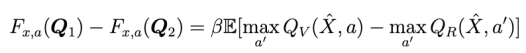
Thus

$|| \bm F(\bm Q_1)- \bm F(\bm Q_2) ||_{\infty} \leq \beta \max_{\hat{x}} | \max_{a} Q_1(\hat{x},a) - \max_{a'} Q_2(\hat{x},a') | \leq \beta || \bm Q_1 - \bm Q_2 ||_{\infty}\, ,$ as required. $\square$

Infinite Time Horizon

One thought on “Infinite Time Horizon”

Leave a comment Cancel reply

Share this:

One thought on “Infinite Time Horizon”

Leave a comment Cancel reply