Poisson process

The Poisson process is a fundamental object in probability. Just as we have a uniform distribution for a single point in an interval, we would like a notion of a “uniform” distribution for a countable set of points in $\mathbb{R}$ . This motivates the Poisson process. We develop this intuition and then give a definition.

Motivation for the Poisson process

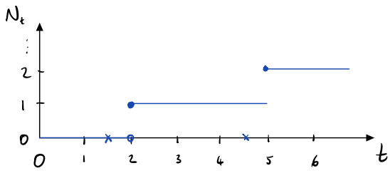
Suppose there is a large town where the probability of a phone call in any given minute is independent, with probability $\lambda$ . We can then count the number of calls in each minute.

Figure: number of calls counted after each minute.

How many minutes are there until the first call occurs? This follows a geometric distribution.

How many calls are there after 10 minutes? This follows a binomial distribution.

Now suppose we divide time into intervals of size $\Delta$ (for example, $\Delta = 1/60$ corresponds to seconds). If we want to keep the average number of calls per minute equal to $\lambda$ , we obtain the following picture.

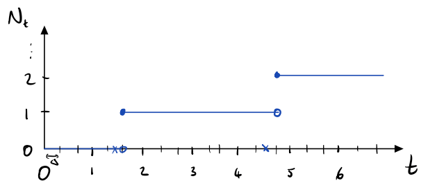
Figure: number of calls counted over intervals of size $\Delta$ .

How much time is there until the first call? This is still geometric:

$\displaystyle \Delta \cdot \text{Geom}(\lambda \Delta)$

How many calls occur after $t$ minutes?

$\displaystyle \text{Bin}(t/\Delta, \lambda \Delta)$

Now let $\Delta \to 0$ .

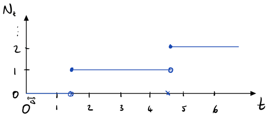
Figure: the limiting continuous-time process.

The geometric distribution converges to an exponential distribution:

$\displaystyle \Delta \cdot \text{Geom}(\lambda \Delta) \;\xrightarrow{\mathcal{D}}\; \text{Exp}(\lambda)$

The binomial distribution converges to a Poisson distribution:

$\displaystyle \text{Bin}(t/\Delta, \lambda \Delta) \;\xrightarrow{\mathcal{D}}\; \text{Po}(\lambda t)$

The resulting process has exponentially distributed waiting times between events, and the number of events in any interval is Poisson distributed.

Poisson process: coin-tossing intuition

The previous example gives useful intuition. Imagine tossing a coin at every point along the real line, where the probability of heads is very small. Each time the coin lands heads, we record a point in our process.

This illustrates two key ideas: