Continuous-time Markov chains

We want to model queueing systems in continuous time. Continuous-time Markov chains are a natural generalization of discrete-time Markov chains. We focus on developing intuition for continuous-time chains as the natural continuous-time extension of discrete chains, similar to our discussion of Poisson processes.

Continuous vs discrete time models

Often, we want to calculate the stationary distribution of a model to summarize long-run behaviour. We saw that using detailed balance equations is convenient for this.

However, detailed balance does not generally hold for discrete-time models, since multiple events can occur simultaneously, complicating the balance equations. Continuous-time models separate these events and are therefore more convenient.

We will also assume that the time spent in each state is exponential. This is reasonable for arrival processes (which are often modeled as Poisson), though it may be less realistic for service times. Nonetheless, this assumption leads to tractable models and useful insights.

Intuition: from discrete to continuous time

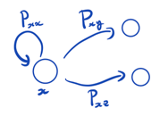
Figure: a discrete-time Markov chain.

The chain jumps to itself with probability $P_{xx}$ and to another state $y$ with probability $P_{xy}$ .

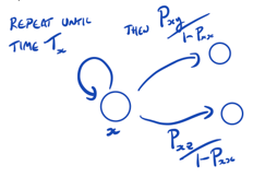
Figure: geometric waiting time interpretation.

That is, the process remains in state $x$ for a geometrically distributed number of steps, and then jumps to state $y$ with probability $P_{xy}$ .

Now suppose we let $P_{xx}$ approach 1 and rescale time appropriately. For small $\Delta$ , define

$\displaystyle P_{xx} = 1 + \Delta Q_{xx}, \quad P_{xy} = \Delta Q_{xy}$

with $Q_{xx} < 0$ and $Q_{xy} > 0$ for $y \ne x$ .

To ensure probabilities sum to 1, we require

$\displaystyle \sum_{y \ne x} Q_{xy} = -Q_{xx}$

As $\Delta \to 0$ , the holding time at state $x$ converges from

$\displaystyle \Delta \cdot \text{Geom}(\Delta q(x))$

$\displaystyle \text{Exp}(q(x))$

while the jump probabilities remain fixed.

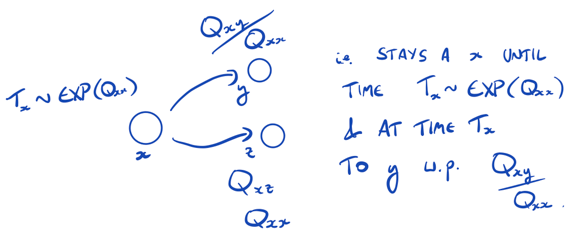
Figure: limiting continuous-time behaviour.

Thus, the process spends an exponential time with parameter $q(x) = -Q_{xx}$ in state $x$ , and then jumps to state $y$ with probability $q(x,y)/q(x)$ .

A formal definition: continuous-time Markov chain

Definition (Q-matrix). A matrix $Q = (q_{xy} : x,y \in \mathcal{X})$ is a Q-matrix if

$q_{xy} \ge 0$ for all $y \ne x$
$q_{xx} = -\sum_{y \ne x} q_{xy}$ for all $x$

Thus, off-diagonal entries are non-negative, diagonal entries are negative, and each row sums to zero. We write $q(x) = -q_{xx}$ and $q(x,y) = q_{xy}$ .

Definition (continuous-time Markov chain). A continuous-time Markov chain is a stochastic process $X = (X(t) : t \in \mathbb{R}_+)$ defined by an initial distribution $\lambda = (\lambda_x)$ and a Q-matrix $Q$ .

The embedded discrete-time chain $Y = (Y_n)$ has transition probabilities

$\displaystyle P_{xy} = \frac{q_{xy}}{q(x)}$

The holding time in state $y$ is

$\displaystyle \tau_n \sim \text{Exp}(q(y))$

The process is constructed via

$\displaystyle X_t = Y_n \quad \text{if} \quad \sum_{k=0}^n \tau_k \le t < \sum_{k=0}^{n+1} \tau_k$

Facts about continuous-time Markov chains

$\displaystyle \mathbb{P}(X_t = x) = [\lambda e^{Qt}]_x$
The matrix exponential is $\displaystyle e^{Qt} = I + tQ + \frac{t^2}{2!}Q^2 + \frac{t^3}{3!}Q^3 + \cdots$
$\displaystyle \mathbb{P}(X(t_{n+1}) = x_{n+1} \mid X(t_n) = x_n, \ldots) = \mathbb{P}(X(t_{n+1}) = x_{n+1} \mid X(t_n) = x_n)$
$\displaystyle \mathbb{P}(X(t+\Delta) = y \mid X(t) = x) = \delta_{xy} + \Delta q_{xy} + o(\Delta)$
The values $q_{xy}$ represent transition rates from $x$ to $y$ , and $q(x)$ is the rate of leaving state $x$ .
Definitions of recurrence, transience, irreducibility, etc., extend naturally (with sums replaced by integrals).