Lai Robbins Lower-Bound

We continue the earlier post on finite-arm stochastic multi-arm bandits. The results so far have suggest that, for independent identically distributed arms, the correct size of the regret is of the order $\log T$ . We now more formally prove this with the Lai and Robbins lower-bound .

We suppose that there are $N$ arms as described at the very beginning of this section. We let $P_a$ be the probability distribution of the rewards from arm $a\in \mathcal A$ . For the Lai and Robbins lower-bound, it is useful to think of $\mathcal A$ as a subset of size $N$ with values from a set of parameters $\Theta$ , i.e. $\mathcal A \subset \Theta$ , and that $P_{\theta}$ is the probability distribution of rewards under the parameter choice $\theta$ . (To be concrete, think of $\Theta$ being the interval $[0,1]$ and $P_\theta$ being a Bernoulli distribution with parameter $\theta$ .)

Asymptotic Consistency. To have a reasonable lower-bound we need to assume a reasonable set of polices. For instance, we need to exclude polices that already know the reward of each arm. Lai and Robbins consider amougst policies that are asymptotically consistent, which means, for each set of arms $\mathcal A$ , for all $a \notin \mathcal A^\star$

$\begin{aligned} \label{RM:e:asymp} \mathbb E [T_a] = o(T^{\eta})\end{aligned}$

(1)

for every $\eta\in (0,1)$ . I.e. a policy is a “good” policy if it can do better than any power $T^\eta$ in playing sub-optimal arms. (Recall here $\mathcal A^\star$ is the set of optimal arms, and $T_a$ is the number of times we play arm $a$ by time $T$ .)

The Lower Bound. The Lai–Robbins Lower Bound is the following:

Theorem [Lai and Robbins ’85]

$\begin{aligned} \liminf_{T\rightarrow\infty} \frac{\mathbb E[T_a]}{\log T} \geq \frac{1}{D(P_a ||P_{\star})}\end{aligned}$

and thus

$\begin{aligned} \liminf_{T\rightarrow\infty} \frac{\mathcal R \! g(T)}{\log T} \geq \sum_{a\in\mathcal A}\frac{\Delta_a}{D(P_a ||P_{\star})}\, \end{aligned}$

where here $D(P_a||P_\star)$ is the Relative Entropy (defined in the appendix) between the distribution of arm $a$ , $P_a$ and the distribution of the optimal arm, $P_\star$ .

For independent rewards $r_1,...,r_t \sim P$ and independent rewards independent rewards $r'_1,...,r'_t \in P'$ , under mild conditions, there exists a function $D(r')$ such that

$\begin{aligned} \label{RM:e:mchange} \mathbb P( (r_1,...,r_t) \in C) = \mathbb E' \left[ e^{\sum_{s=1}^t D(r'_s)} \mathbb I [(r_1,...,r_t) \in C] \right]\end{aligned}$

(2)

and

$\begin{aligned} \label{RM:e:mean} D(P||P') = \mathbb E [ D(r)]\, .\end{aligned}$

(3)

(The term is $e^{D(r)}$ is just the ratio between $P(r)$ and $P'(r)$ and is formally called Radon-Nikodym derivative.) For the Lai Robbins lower-bound, we also require the assumption that

$D(P|| P_{a'}) \rightarrow D(P || P_{a})$

as $a' \rightarrow a$ . This is required to get the constants right in the theorem but is not critical to the overall analysis.

We now prove the Lai and Robbins Lower-bound.

Proof. We take an increasing sequence of integers $n_T$ . We will specify it soon but for now it is enough to assume that $n_T=o(T)$ . We can lower-bound the expected number of times arm $a$ is played as follows:

(4)

Here we see that we want to take $n_T$ as large as possible while keeping the probability $\mathbb P(T_a \leq n_T)$ away from $1$ . When arm $a$ was replaced by an arm $a'$ whose mean reward is the larger than each arm in $\mathcal A$ (i.e. $\bar r' > r_{\star}$ ) then we can analyze this probability:

$\begin{aligned} \label{RM:e:pb} \mathbb P'(T_{a'} \leq n_T) = \mathbb P' (T-T_{a'} \geq T- n_T) \leq \frac{ \mathbb E[ T- T_{a'} ] }{ T-n_T } = \frac{ o(T^{\eta})}{T-n_T} = o(T^{\eta-1})\, .\end{aligned}$ (5)

In the inequality above we apply Markov’s Inequality and the asymptotic consistency assumption . (Note the above bound holds for every $\eta \in (0,1)$ so in informal terms we could think of the above bound as being $O(T^{-1})$ .)

We can change arm $a$ for arm $a'$ through the change of measure given above in . This involves the sum of independent random variables $\sum_{k=1}^{n_T} D(r_k)$ which by and the weak law of large numbers satisfies:

Here we apply the shorthand $P=P_a$ and $P'=P_{a'}$ .

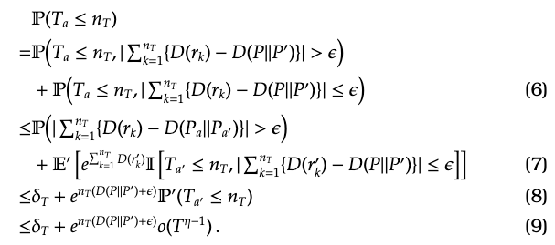
We now have various pieces in place where we can now analyze the probabilities $\mathbb P ( T_a \leq n_T)$ as follows:

In the first equality (6), we split the probability according to how close $\sum_{k=1}^{n_T} D(r_k)$ is to $n_T D(P||P')$ . In the inequality (7), we remove the condition $\{T_a \leq n_T\}$ from the first term and apply the change of measure to the second term (2). The condition on $\sum_{k=1}^{n_T} D(r_k)$ and the definition of $\delta_T$ yields (8). Finally follows from the bound on $\mathbb P'(T_{a'} \leq n_T)$ given in (5).

So, we have

$\begin{aligned} P(T_a \leq n_T) \leq \delta_T + e^{n_T (D(P||P')+\epsilon)} \mathbb P'(T_{a'} \leq n_T)\end{aligned}$

and recall we want the probability above to stay away from $1$ . The only term that can grow is in the exponent $e^{n_T (D(P||P')+\epsilon)}$ . So the largest we can make $n_T$ without this growing is by taking

$n_T = (1-2\eta) \frac{\log (T)}{D(P||P')+\epsilon} \, .$

This gives

$\begin{aligned} P(T_a \leq n_T) \leq \delta_T + o(T^{-\eta})=o(1)\,.\end{aligned}$

which applied to the bound (4) gives

$\begin{aligned} \mathbb E [T_a] \geq n_T( 1- o(1)) = (1-2\eta) \frac{\log (T)}{(D(P||P')+\epsilon)}( 1- o(1))\end{aligned}$

Thus

$\begin{aligned} \liminf_{T\rightarrow\infty} \frac{\mathbb E [T_a] }{\log T} \geq \frac{1}{D(P||P_\star)}\end{aligned}$

which is the required bound on $\mathbb E[T_a]$ . (Some technical details: Here after taking the limit we set $\eta$ to zero, $\epsilon$ to zero and set $P'$ to $P_{\star}$ . We can do this because the bound holds for all $\eta>0$ and $\epsilon>0$ . Also $a'$ is an arbitrary parameter such that $r' > r_\star$ so we apply our assumption that $D(P_{a} || P_{a'}) \rightarrow D(P_a || P_{\star})$ as $a' \rightarrow a^\star$ .)

Finally, for the regret bound we recall that

$\begin{aligned} \mathcal R\! g(T) = \sum_{a\notin\mathcal A^\star} \Delta_a \mathbb E [ T_a] \end{aligned}$

Thus applying the bound on each term $\mathbb E[T_a]$ gives the regret bound

$\begin{aligned} \liminf_{T\rightarrow\infty} \frac{\mathcal R \! g(T)}{\log T} \geq \sum_{a\in\mathcal A}\frac{\Delta_a}{D(P_a ||P_{\star})}\, .\end{aligned}$