Euler-Maruyama

The Euler-Maruyama scheme is a method of approximating an stochastic differential equation. Here we investigate two forms of error the scheme: the weak error and the strong error. The aim is to later we will cover Multi-Level Monte Carlo (MLMC) and related topics.

Euler. Let’s quickly recall the standard, Euler scheme: for an o.d.e.

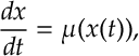
the Euler approximation is

for $t=0,h,2h,...$ . I.e. you make steps of size $h$ .

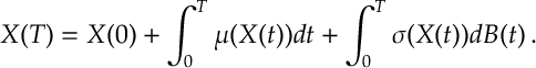
Euler-Maruyama. The Euler-Maruyama scheme is a natural extension of this. For an s.d.e.

the Euler-Maruyama scheme is

for $t=0,h,2h,...$ . Here $B^{(h)}(t)$ is independent normally distributed with mean $0$ and variance $h$ .

Weak Error and Strong Error. The weak error at time $T$ for a (Lipschitz) function $f$ is

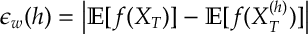
(Note this is really the $L_1$ distance between $X_T$ and $X_T^{(h)}$ .) The strong error is

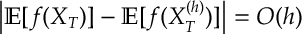
Main Result. We prove the following

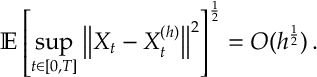
Theorem. Given $\mu$ and $\sigma$ are bounded and Lipschitz continuous then, for the Euler-Maruyama Scheme, for $X_t$ real-valued, the weak error satisfies

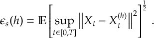
and the strong error satisfies

Proof. In the proof, we will make good use of the twos facts:

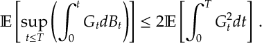
and

The first is an application of Doob’s $L^2$ inequality and Itô’s isometry and the second is Gronwall’s Lemma.

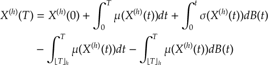
We analyze the strong error. We define $\lfloor t \rfloor_h = \max \{ h k : hk \leq t \}$ . Note that

where as

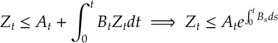
The only difference between the two expressions deducted in . We use Gronwall’s Lemma to investigate the impact of these two terms. Thus

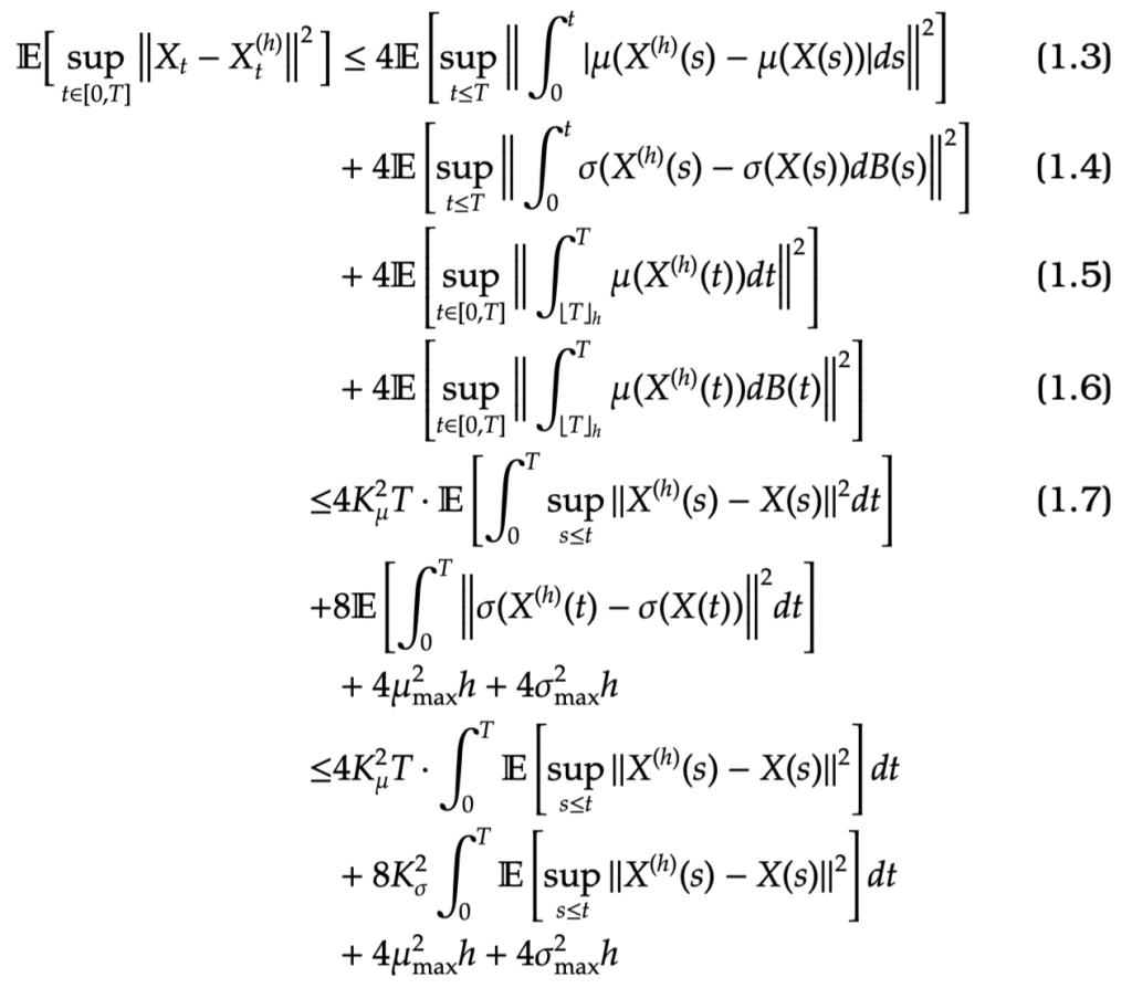
There are lots of small (but standard) changes going on in the expressions above. In the first inequality above we use the fact that $(a+b+c+d)^2\leq 4a^2+4b^2 + 4 c^2 + 4 d^2$ . For the term (1.7) from (1.3) , we apply the Lispchitz property of $\mu(\cdot)$ , then we apply Jensen’s inequality to take the square inside the integral (thats where the $T$ comes from in (1.7) ), then we take the supremum inside the expectation. For (1.7) from (1.4), we apply the Itô isometry from above. For (1.5) and (1.6), we use the boundedness of $\mu$ and $\sigma$ . Then in the third inequality, we apply the Lipschitz property to $\sigma(\cdot)$ then we take a supremum side the integral.

Notice in the end we see that

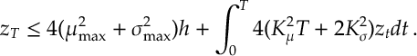
Thus by Gronwall’s Lemma

Thus taking a square root gives the required result.

We analyze the weak error. We note that if $X(t)$ is real-valued then

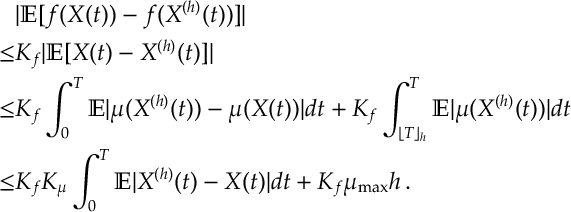
[The first bound works for real valued $X$ since $f(X) - f(Y) \leq K (X-Y)$ .] Applying Gronwall’s Lemma again

Thus,

QED

References.

Proofs of convergence for the Euler-Maruyama method can be found in Bally & Talay. The book of Kloeden and Platen proof of weak and strong convergence (though I am yet to get hold of a copy). Note the proof above follows well established lines for proving path-wise uniqueness of SDEs. Giles keeps good slides on his website surveying the area and has recent proofs removing the Lipschitz assumptions. An alternative approach that improves on Euler-Mayurama is Milstein \cite{mil1975approximate} and I will develop the notes in this direction in due course.

Bally, Vlad, and Denis Talay. “The Euler scheme for stochastic differential equations: error analysis with Malliavin calculus.” Mathematics and computers in simulation 38.1-3 (1995): 35-41.

Bally, Vlad, and Denis Talay. “The law of the Euler scheme for stochastic differential equations: II. Convergence rate of the density.” (1995).

Kloeden, Peter E., and Eckhard Platen. Numerical solution of stochastic differential equations. Vol. 23. Springer Science & Business Media, 2013.

Mike Giles: http://people.maths.ox.ac.uk/~gilesm/

Mil’shtejn, G. N. “Approximate integration of stochastic differential equations.” Theory of Probability & Its Applications19.3 (1975): 557-562.

References.

Share this:

Like this:

Leave a Reply Cancel reply