Inventory Control

We consider the problem where there is an amount of stock $x_t$ at time $t$ . You can perform the action to order $a_t$ units of stock. Further the demand at time $t$ is $d_t$ . We assume $d_t$ is independent over $t$ . The change in the amount of stock follows the dynamic:

$\begin{aligned} x_{t+1} = x_t + a_t -d_t \,.\end{aligned}$

It is possible for $x_t$ to be negative, which corresponds to backordered stock.

There is a cost for ordering $a \in \mathbb R$ units of stock:

$c(a) = K+ c a \, .$

Note here $c(a)=0$ if $a=0$ . There is a cost $\kappa(x)$ for holding stock when $x>0$ or for unmet demand when $x<0$ . Specifically

$\begin{aligned} \kappa(x) = \begin{cases} p x &\text{if } x\geq 0\, , \\ h x & \text{if } x < 0 \,. \end{cases}\end{aligned}$

for positive constants $h$ and $p$ . If we consider the minimization problem over $T$ time steps then we have a dynamic program:

$\begin{aligned} L_T(x) = \min_{a_0,...,a_T} \mathbb E \left[ \sum_{t=0}^T c(a_t) + \kappa(x_t+a_t - d_t) \right] \, .\end{aligned}$

The Bellman equation for this optimization problem is

$\begin{aligned} L_{t}(x) & = \min_{a\geq 0} \{ c(a) + \mathbb E_d [ \kappa (x+a-d) ] + \mathbb E [L_{t-1}(x+a - d)] \} \\ & = \min_{y\geq x} \{ c(y) + \mathbb E_d [ \kappa (y-d) ] + \mathbb E [L_{t-1}(y - d)] \} - c x \, .\end{aligned}$

Here $y=x+a$ . If we define $B(x)$ as follows

$\begin{aligned} B_t(y) = cy + \mathbb E_d [ \kappa (y-d) ] + \mathbb E [L_{t-1}(y - d)] \, ,\end{aligned}$

then (removing the subscript $t$ for now) notice the above Bellman Equation becomes

$\begin{aligned} \label{sS:LOpt} L(x) = \min \Big\{ B(x) , \min_{y > x} \, \{K + B(x) \} \Big\} - cx\, .\end{aligned}$

There exists an explicit closed form solution to this optimization. Specifically there exists values $s$ and $S$ such that if the stock level goes below $s$ then we order enough to have $S$ units of stock. (We will show that $S$ minimizes $B(x)$ and $s$ is such that $B(s) = K+B(S)$ .)

We give a proof for the case where $K=0$ . This gives the necessary intuition for the more general case where $K>0$ , which we subsequently discuss. (The formal argument is given in a series of exercises: Ex 2–Ex 4.)

$S$ -Inventory control.

We consider the equation with $K=0$ . Notice if $B(x)$ is convex and $B(x) \rightarrow\infty$ as $|x|\rightarrow\infty$ then $S$ , the minimum of $B$ , is finite. Thus from it holds that:

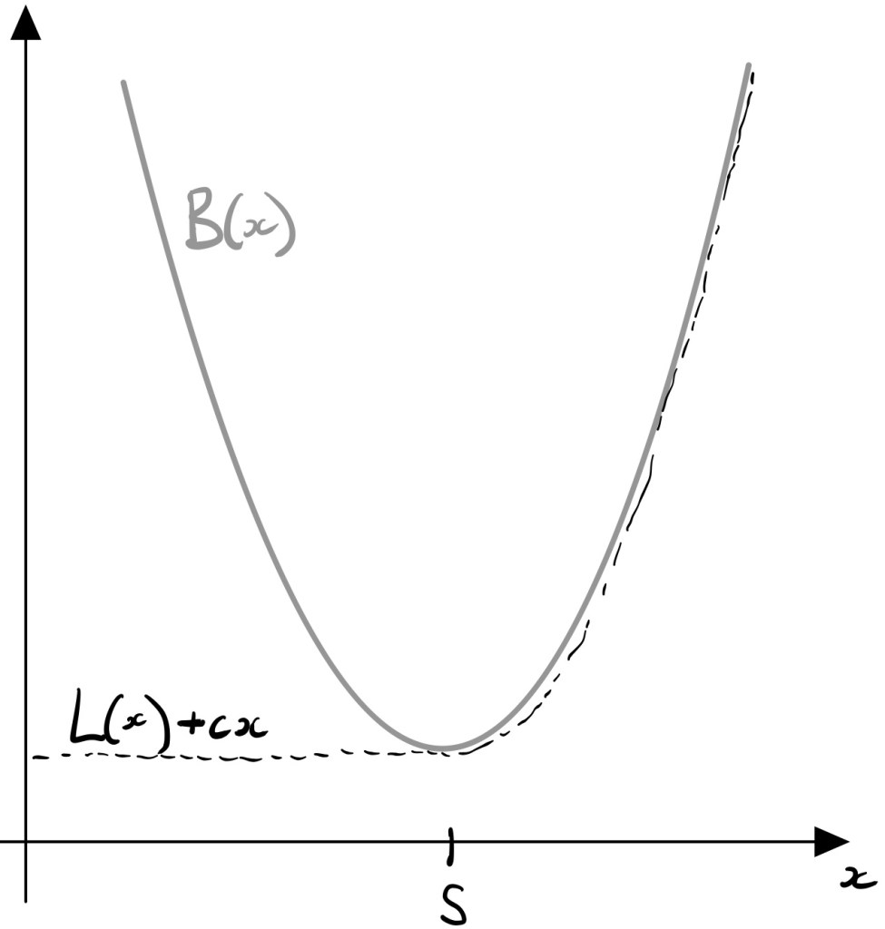
$\begin{aligned} L(x) + c x = \min_{y \geq x} B(y) = \begin{cases} B(S) & \text{if } x \leq S\, , \\ B(x) & \text{if } x > S\, . \end{cases}\end{aligned}$

Notice if $B(x)$ is convex then relatively straight forward to check that $L(x)$ is convex and $L(x)\rightarrow\infty$ and $|x| \rightarrow \infty$ (see Ex [sS:Ex0]). Also see the following Figure:

Figure: $B(x)$ and $L(x)$ for $K=0$ .

Further, if, given the function $L(x)$ above, we now update $B(x)$ by taking

$\begin{aligned} B(y) = cy + \mathbb E_d [ \kappa(y-d) ] + \mathbb E_d [ L(y-d) ] \, ,\end{aligned}$

then it is straight-forward to check that the new function $B$ is also convex and $B(x)\rightarrow \infty$ as $|x| \rightarrow\infty$ (see Ex [sS:Ex0]).

Thus (putting sub-script $t$ back and noting that $L_0(x)$ is convex) we see that the sequence of functions $L_t(x)$ and $B_t(x)$ are convex and that $S_t$ , the minimum of $B_t(x)$ , defines the optimal control

If $x < S_t$ then order so you have $S_t$ units of stock, $x+a = S_t$ .
If $x \geq S_t$ then do nothing.

$(s,S)$ -Inventory control.

We consider the equation with $K>0$ . That is

$\begin{aligned} \label{sS:L2} L(x)+cx = \min \Big\{ B(x) , \min_{y > x} \, \{K + B(x) \} \Big\} \, .\end{aligned}$

In general $B(x)$ will not be convex, but let’s assume it is for a moment in order to gain intuition. Again let $S$ be the minimum of $B(x)$ . In this case the minimization over $y >x$ above is solved at $y=S$ if $x\leq S$ and $y=x$ if $x>S$ . (Note if $y=x$ in it is obviously better to take $B(x)$ rather than $B(x)+K$ .) So we have that

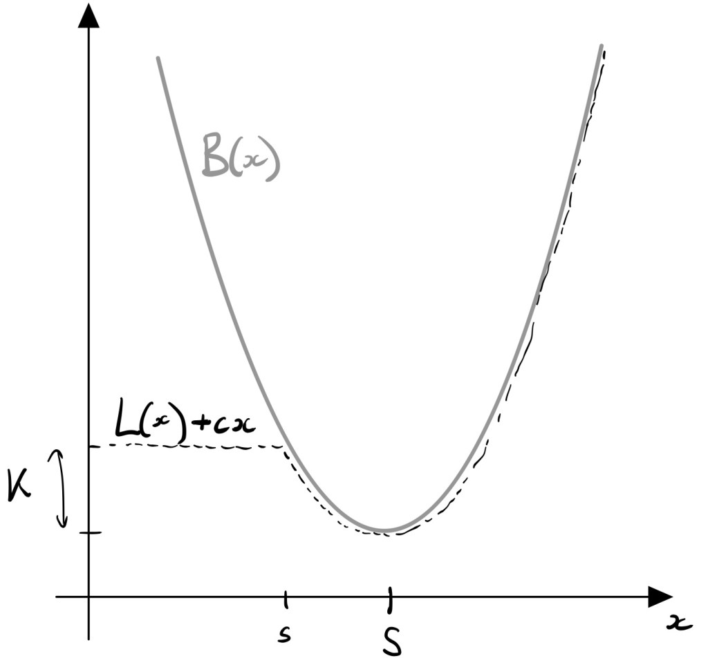
$\begin{aligned} \label{sS:L} L(x) + cx = \min\left\{ B(x), K+B(S)\right\} \, .\end{aligned}$

Now assuming $B(x)$ is continuous then there will be a value of $x=s < S$ such that $\begin{aligned} \label{sS:s} B(s) = K+B(S) \,. \end{aligned}$ This will be the point for which for $x < s$ then $K+B(S)$ is the minimum in , while for $x \geq s$ , $B(x)$ will be the minimum in . I.e. In this case the optimal control will be

$\begin{aligned} \label{sS:x} x+a= \begin{cases} S &\text{if } x < s \, , \\ x &\text{if } x \geq s \, . \end{cases}\end{aligned}$

For a convex function $B(x)$ we plot $L(x) +ca$ in Figure [sS:Fig2]. Notice that $L(x)$ is clearly not convex. Essentially, the additional $K$ term has introduced a “bump” of size $K$ . So rather than assume convexity motivates, this motivates the idea of $K$ -convexity.

Fig: $B(x)$ and $L(x)+cx$ for $K>0$ .

Definition [ $K$ -convex] A function $B$ is $K$ -convex if

$\begin{aligned} {K}+ B(z+y) \geq B(z) + z\left[ \frac{B(y) - B(y-b)}{b} \right] \end{aligned}$

Remark. The definition above is not terribly intuitive. It can be shown that $K$ -convexity means that for $x<z$ the line segment from $(z,B(z)+K)$ to $(x,B(x))$ does not intersect $(y,B(y))$ for any value of $y$ between $x$ and $z$ . I.e. if you are standing at point $(z,B(z)+K)$ you have an unobstructed view of $(x,B(x))$ .

If $B(x)$ is $K$ -convex then we can show that is solved by , just like in the convex case. (This is Ex [sS:Ex1].) Further, we can show that if $B(x)$ is $K$ -convex then $L(x)$ defined by is $K$ -convex. (This is Ex [sS:Ex3]). Thus it can be shown that when we update $B(x)$ according to the rule

$\begin{aligned} B(y) = cy + \mathbb E_d [ \kappa (y-d) ] + \mathbb E [L(y - d)]\end{aligned}$

then $B$ is also $K$ -convex. (This is Ex [sS:Ex2].)

Exercises

Ex 1. a) Given $B(x)$ is convex and $B(x) \rightarrow\infty$ for $|x|\rightarrow\infty$ , show that

$\begin{aligned} L(x) + c x = \min_{y \geq x} B(y) = \begin{cases} B(S) & \text{if } x \leq S\, , \\ B(x) & \text{if } x > S\, . \end{cases}\end{aligned}$

is such that $L(x)$ is convex and $L(x) \rightarrow\infty$ for $|x|\rightarrow\infty$ .
b) Given $L(x)$ is convex and $L(x) \rightarrow\infty$ for $|x|\rightarrow\infty$ , show that

$\begin{aligned} B(y) = cy + \mathbb E_d [ \kappa(y-d) ] + \mathbb E_d [ L(y-d) ] \, ,\end{aligned}$

is such that $B(x)$ is convex and $B(x) \rightarrow\infty$ for $|x|\rightarrow\infty$ .

Ex 2. We let $B(x)$ be $K$ -convex, continuous with $B(x) \rightarrow \infty$ as $|x|\rightarrow\infty$ . Also let $S= \min B(x)$ and $s$ is the smallest number such that $B(s) = B(S) + K$ .
a) Show that, for $x < s$ , $B(x) > B(S)+K$ .
(Hint: show $B(x) > B(s)$ .)
b) Show that for $s < x<y$ , $B(x) \leq B(y)+K$ .
(Hint: consider two cases $x<S$ and $x>S$ .)
c) Show that :

$\begin{aligned} L(x)+cx = \min \Big\{ B(x) , \min_{y > x} \, \{K + B(y) \} \Big\} \, \end{aligned}$

is solved by :

$\begin{aligned} x+a= \begin{cases} S &\text{if } x < s \, , \\ x &\text{if } x \geq s \, . \end{cases}\end{aligned}$

The following exercise establishes some properties of $K$ -convex functions

Ex 3. Show that
a) The sum of $K$ -convex functions is $K$ -convex.
b) A convex function is $K$ -convex.
c) If $B(x)$ is $K$ -convex then so is $B(x+a)$ is $K$ -convex.
d) The convex combination of $K$ -convex functions is $K$ -convex.
e) If $B$ is $K$ -convex then $\mathbb E_Z [ B(x+ Z)]$ is $K$ -convex.

Ex 4. If we let

$\begin{aligned} L(x) = \begin{cases} K + B(S) - cx &\text{if } x < s\, , \\ B(x) - cx & \text{if }x \geq s \, . \end{cases}\end{aligned}$

where $S$ minimizes $B(x)$ and $s$ is the smallest value such that $B(s) = K + B(S)$ . We will show that $L$ is $K$ -convex:

$\begin{aligned} \label{sS:KCEx} {K}+ L(z+y) \geq L(z) + z\left[ \frac{L(y) - L(y-b)}{b} \right] \,.\end{aligned}$

Verifying by moving $s$ through the following cases:
a) $s \leq y-b$
b) $y-b <s < y$ and $B(y) \geq B(s)$
c) $y-b <s < y$ and $B(y) < B(s)$
d) $y < s < y+z$
e) $y+z <s$

References.

The idea of $K$ -convexity is due to Scarf. A full account of all the calculations above is given in the excellent text of Bertsekas.

Scarf, Herbert. “The optimality of (5, 5) policies in the dynamic inventory problem.” Optimal pricing, inflation, and the cost of price adjustment (1959).

Bertsekas, Dimitri P. Dynamic programming and optimal control. Vol. 1. No. 2. Belmont, MA: Athena scientific, 1995.