Stochastic Finite Arm Bandits

We discuss a canonical multi-arm bandit setting. The stochastic multi-arm bandit with finite arms and bounded rewards. We let $a=1,...,N$ index the set of arms. We let $\mathcal A=\{1,...,N\}$ be the set of arms. If you play the arm $a$ at time $t\in\mathbb N$ , you receive rewards $r_t(a)$ which are independent and identically distributed in $t$ . However, the distribution between arms may change.

We let $\bar r(a)$ be the mean of arm $a$ . We want to find the machine with highest mean reward.

We define

and also we define

We do not know these averages in advance and we only know the rewards from the times that we play each machine – we are only allowed to play one machine per unit time.

We let $\hat r_t(a)$ denote the empirical mean of arm $a$ after it has been played $t$ times. Given the central limit theorem and the Azume-Heoffding bound (see appendix), we can assume the following

Assumption. There is some function $\Lambda(\Delta)$ positive for $\Delta>0$ such that

Many reasonably behaved distributions obey this condition. For instance, any bounded random variable and Gaussian random variables. This assumption can be relaxed.

A policy chooses a sequence of arms, $\pi_t$ at times $t\in\mathbb N$ as a function of the rewards previously experienced, i.e. as a function of $\{ \pi_s, r_s(\pi_s) \}_{s=1}^{t-1}$ . As with MDPs, the expected cumulative reward of policy $\pi$ at time $T$ is

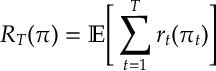
Def. [Regret] The regret of policy $\pi= \{\pi_t\}_{t=1}^T$ at time $T$ is¹

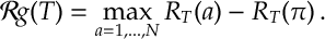
The regret is a frequently used metric of choice for bandit problems and many other areas of statistical learning.

The following lemma shows that we can analyse the regret by understanding the number of times we play a sub-optimal arm or equivalently calculating the probability that we play a sub-optimal arm.

Lemma [SMAB:Lem1] For a multi-arm bandit problem with Bernoulli rewards

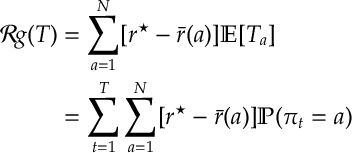
where $T_a$ is the number of times arm $a$ is played by time $T$ .

Proof. We can expand the reward of the optimal arm with

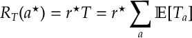
and, by independence, we can replace the reward with its expectation as follows

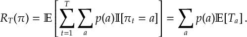
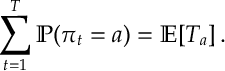
Now subtracting from gives the regret and the first equality. The second equality follows immediately from the fact that

QED.

Explore and Commit.

Explore and commit gives a simple way of understanding the explore-exploit trade-off and why a regret of $O(\log T)$ is achievable.

Suppose we implement the following policy:

Explore-and-Commit.

We play each arm $t$ times.
We play the best arm there after.

Given we are going to run our bandit experiment for $T$ rounds, we now look for a good choice of $t$ .

Theorem. For $t=C \log T$ , the regret of explore-and-commit is

In the above, notice we need $C\Delta^2/c> 1$ to get good results for large $T$ and we don’t know $\Delta$ in advance. This is a weakness.

Proof. Let $A^\star = \{ a : r(a) = \max_{a'} r(a') \}$ be the set of optimal arms. For any $a \notin A^\star$ and $a^\star \in A^\star$ , I.e. either $a$ or $a^\star$ must observe rewards away from their expected mean for $a$ to beat $a^\star$ in the explore phase.

We can split the regret into its explore and commit phases and then apply the above inequality:

(At this point it is worth noting that the term in square brackets can easily be minimized, and it is minimized at $t= (c/\Delta^2) \log (4 \Delta^2T/c)$ . So basically $t=O(\log T)$ is the right amount of exploration.) Substituting in $t= C\log T$ to the term in square brackets gives the result.

QED.

Deterministic Exploration.

The exploration phase in explore and commit does not have to all happen that the beginning. An easy way to deal with exploration is to decide in advance when you are going to explore each arm.

Specifically, for each arm $a$ take $E_a(t)\in \mathbb Z_+$ where $E_a(t)$ gives the number of times arm $a$ is explored by time $t$ .²

Deterministic Exploration. At time $t$ ,

If $E_a(t) > E_a(t-1)$ play arm $a$ .
If no such arm exists, play the arm with highest reward found during exploration.

If $E_i(T) \sim C_T \log T$ where $C_T$ is a slowly increasing function (think $C_T= \log (e+ \log (T))$ ) then a very similar proof to the explore and commit proof gives

This is an exercise.

Epsilon-Greedy.

Rather tracking how long you need to play each arm a simple heuristic, with a similar proof to deterministic exploration is to randomize.

$\epsilon$ -Greedy. At time $t$

with probability $\epsilon_t$ , play an arm uniformly at random.
Else, with probability $1-\epsilon_t$ , play the arm with highest reward.

The proof for this policy is very similar to the deterministic exploration case. (We just need to apply a [Bernstein] concentration bounds to the amount of exploration.) Similar to before if $\epsilon_t = C_t/t$ for a slowly increasing function then

Again this is an exercise for the reader.

At this point, it is worth noting that we can get arbitrarily close to $\log T$ with bounds and simple policies. So the moral of the story so far is: no matter what you do, as long as you explore every arm a bit more that $\log T$ times and you spend the rest of your time on the best arm seen so far then you should have a good regret bound.

As we see shortly, with the Lai-Robbins lower bound, $\mathcal R\!g(T) =O(\log T)$ is the right rate of convergence for regret in the stochastic setting. We can also achieve this bound with a policy called Upper-Confidence Bound (UCB). The idea is to construct a statistical confidence bound and then choose the arm with confidence bound (empirical mean plus confidence error). UCB is a fantastic policy used all over the place. However, it should be noted that in practice it does not always generalize. Thus one should fall back on simpler policies, remembering the rules of thumb developed so far.

Upper Confidence Bound.

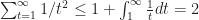
The proofs so far have relied on the bound

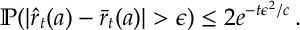
We noted that if we take $t \approx \log T$ then the probability of choosing the wrong arm goes down very fast and does not contribute to the regret bound. Basically, the regret of $\log T$ occurs because of the $t \approx \log T$ arm pulls that were required to get the concentration in the first place.

Based on this, the Upper Confidence Bound algorithm looks at the values of $\epsilon$ that guarantee this fast decay in probability. It assesses how confident are we about each estimate on the mean and then chooses the arm with highest mean plus error. Specifically, for $t$ and $t_a \leq t$ , we define $\epsilon_{t_a,t}$ to be such that

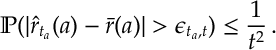
Given this holds for $\epsilon$ such that

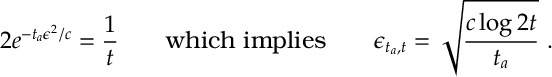
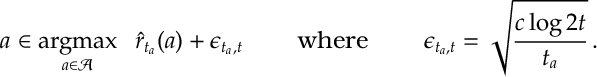
From now on we will take $\epsilon_{t_a,t}$ as given above, where $t$ is the number of rounds of the algorithm and $t_a$ is the number of times arm $a$ has been selected by time $t$ .

UCB choses the highest empirical mean plus error:

Upper-Confidence Bound (UCB).

Choose any arm such that

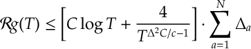
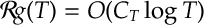
Notice for UCB algorithm so long as arm $a$ is not played the $\log t$ will deterministically keep increasing (and eventually) will dominate forcing the policy to explore $a$ . Notice we need to monitor what is going on with all arms at all times implement an iteration of UCB. The following result shows that we get a much more crisp regret bound for UCB.

Theorem. The regret of UCB is

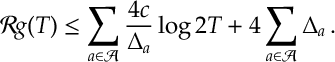
Proof. Given Lemma [SMAB:Lem1], we investigate the probability that UCB might select a sub-optimal arm. We will see that it occurs either because of insufficient exploration (which we will see is an issue that can only occur a small –order $\log T$ – number of times) or because of insufficient concentration (which is unlikely to happen because of the way we cooked-up $\epsilon_{t_a,t}$ ).

Specifically, suppose at time $t$ the policy chooses $\pi_t=a$ for $a \notin \text{argmax} \bar r(a')$ then

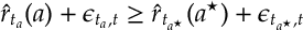
where $a^\star$ is some arm in $\text{argmax} \bar r(a')$ .

In additional to playing arm $a$ at time $t$ , let’s first suppose that both arms are concentrated about their means. Specifically, the following event holds

Then using the bounds in $E_t$ to replace $\hat r$ with $\bar r$ in implies that

which³ in turn implies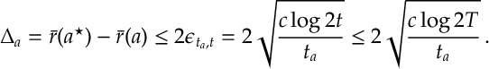

So we have a bound on how much we explored arm $a$ :

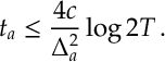
We can interpret this as saying: when we have good concentration, we choose the wrong arm, $a$ , because the amount of exploration $t_a$ was too small. And critically we can see what the right amount of exploration for UCB is quantified in .

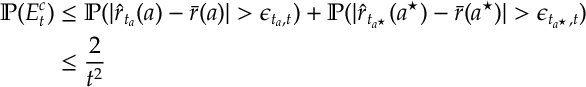
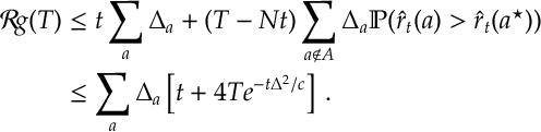
Now we can also bound the probability that the event $E$ does not hold. That is, we a union bound and , we have

Putting everything together,

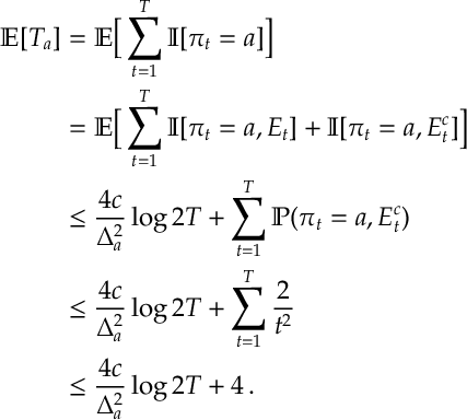
In the first inequality above apply , i.e. there can be at most $\frac{4c}{\Delta^2_a} \log 2T$ times where $a$ is played and $E_t$ holds. In the second inequality we apply [after noting that $\mathbb P ( \pi_t= a, E_t^c) \leq \mathbb P (E_t^c)$ ]. In the final inequality, we use the fact that $\sum_{t=1}^\infty {1}/{t^2} \leq 1+ \int_1^\infty \frac{1}{t} dt =2$ .

The result then follows by applying the above bound to the identity in Lemma [SMAB:Lem1], that is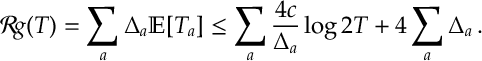

QED.

References.

There are quite a few great sources to go for Bandits. [This post is me revising really as I might teach some bandits next semester.] The reviews of Bubeck & Cesa-Bianchi, Lattimore & Szepesvari and Slivkins all give good coverage. Also there are associated blogs [I am a bandit] and [bandit alas]. The paper of Auer et al. provided a primary source for the above. Epsilon greedy and bandits are discussed in Sutton and Barto’s classic text.

Regret Analysis of Stochastic and Nonstochastic Multi-armed Bandit Problems. Sébastien Bubeck, Nicolò Cesa-Bianchi (https://arxiv.org/abs/1204.5721)
Bandit algorithms by Tor Lattimore and Csaba Szepesvari. 2020 [CUP]
Introduction to bandits by Alex Slivkins
https://blogs.princeton.edu/imabandit/
https://banditalgs.com
Finite-time Analysis of the Multiarmed Bandit Problem. Auer, Cesa-Bianchi & Fischer. Machine Learning volume 47, pages235–256(2002)
Reinforcement Learning: An Introduction. Richard S. Sutton and Andrew G. Barto. http://www.incompleteideas.net/book/the-book-2nd.html

Note the regret depends on the policy, but for convenience we do not explicitly include this in our notation when it is clear what policy is being considered.↩
Here we require that $\sum_a (E_a(t)-E_a(t-1))\in \{0,1\}$ .↩
Note we are fortunate that we don’t need to know $\epsilon_{t_{a^\star},t}$ in the above bound.↩

Explore and Commit.

Deterministic Exploration.

Epsilon-Greedy.

Upper Confidence Bound.

References.

Share this:

Like this:

Leave a Reply Cancel reply