Bayesian Online Learning

We briefly describe an Online Bayesian Framework which is sometimes referred to as Assumed Density Filer (ADF). And we review a heuristic proof of its convergence in the Gaussian case.

Bayes Rule gives

$p(\theta | D_{t+1} ) = \frac{ P(y_{t+1} |\theta) p(\theta |D_t) }{ \int P(y_{t+1} |\theta) p(\theta |D_t) d \theta }$

For data $D_t$ , parameter $\theta$ and new data point $y_t$ .

ADF suggests projecting data at time $t$ to a parameter (vector) $par(t)$ . This gives a routine that consists of the following two steps. (See [Opper] for the main reference article)

Update:

$p(\theta | y_{t+1}, par(t) ) = \frac{ P(y_{t+1} |\theta) p(\theta | par(t) ) }{ \int P(y_{t+1} |\theta) p(\theta |D_t) d \theta }$

Project:

$\min_{par} \quad D_{KL} ( p(\cdot | y_{t+1}, par(t) ) || p(\cdot | par) )$

Here $D( p|| q)$ is the KL-divergence of distributions $p$ and $q$

Remark. Note that for exponential families of distributions:

$p(\theta | par ) \propto \exp \left\{ - \sum_k \alpha_k f_k(\theta) \right\}$

then matching moments of $\mathbb E_{\theta} f_k(\theta)$ gives the minimization of the above.

Let’s assumes that $p(\theta,par)$ is a normally distributed with mean $\hat \theta$ and covariance matrix $C$ .

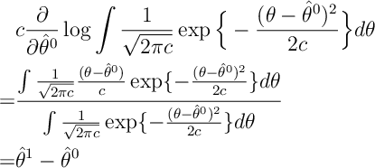
Under this one can argue that $\hat \theta$ obeys the recursion

(1)

$\label{Opper:1} \hat \theta_i (t+1) - \hat \theta_i (t) = \sum_j C_{ij}(t) \partial_j \log \mathbb E_u [ P(y_{t+1} | \hat \theta (t) + u ) ]$

and $C(t)$ obeys the recursion:

(2)

$\label{Opper:2} C_{ij}(t+1) = C_{ij}(t) + \sum_{kl} C_{ik}(t) C_{lj}(t) \partial_k \partial_l \log \mathbb E_u [P(y_{t+1} | \hat \theta (t) + u) ]\, .$

Here $u$ is normal with mean zero and covariance $C(t)$ . The partial derivative, $\partial_j$ , above is taken with respect to the $j$ th component of $\hat \theta(t)$ .

Quick Justification of (1) and (2)

Note that

$\begin{aligned} &c \frac{\partial}{\partial \hat \theta^0} \log \int \frac{1}{\sqrt{2\pi c}} \exp \Big\{ - \frac{(\theta - \hat \theta^0)^2 }{2c} \Big\} d\theta \\ = & \frac{ \int \frac{1}{\sqrt{2\pi c}} \frac{(\theta - \hat \theta^0 )}{c} \exp \{ - \frac{(\theta - \hat \theta^0 )^2}{2c} \} d\theta }{ \int \frac{1}{\sqrt{2\pi c}} \exp \{ - \frac{(\theta - \hat \theta^0 )^2}{2c} \} d\theta } \\ = & \hat \theta^1 - \hat \theta^0\end{aligned}$

A similar calculation gives the other expression on $C$ .

For

$V_{kl} = \partial_k \partial_l \log \mathbb E_u [P(y_{t+1} | \hat \theta (t) + u) ]$

This gives the differential equation

$\frac{d C}{dt} = CVC$

This implies

$\frac{dC^{-1}}{dt} = -V$

because
$0 = \frac{d C C^{-1}}{dt } = C \frac{d C^{-1}}{d t} + \frac{dC}{dt} C^{-1} \quad\implies \quad \frac{dC^{-1}}{dt} = - C^{-1} \frac{d C}{dt} C^{-1} = -V$

We assumes $y$ is drawn IID from a distribution $Q(y)$ . We assumes there is an attractive fixed point $\theta^*$ satisfying

(3)

$\label{Opper:4} \int Q(y) \partial_i \log P(y|\theta^*) dy = 0$

$\begin{aligned} \lim_{t\rightarrow\infty} \frac{C^{-1}(t)}{t} & = \lim_{t\rightarrow\infty} \frac{1}{t} \int^t_0 V(s) ds \\ &= \mathbb E_Q [ \partial_k \partial_l \log \mathbb E_u [P(y_{t+1} | \theta^* + u) ] ] \\ &\approx \mathbb E_Q [ \partial_k \partial_l \log \mathbb E_u [P(y_{t+1} | \theta^* ) ] ] = J(\theta^*)\end{aligned}$

The last approximation that removes the normal distribution error needs justifying. The inequality with $J(\theta^*)$ assumes that $Q(y) = P(y | \theta^*)$ (in the case where they are not equal – i.e. when the model is miss specified – we just puts in some matrix $A$ instead of $J(\theta^*)$ )

In principle $J(\theta^*)$ should not be too far from $J(\theta^*+u)$ , because

$\lim_{t\rightarrow\infty} \frac{C^{-1}(t)}{t} = const \quad\text{and}\quad \lim_{t\rightarrow\infty} \left( t C(t) \frac{C^{-1}(t)}{t} \right) = I$

imply that

$\lim_{t\rightarrow\infty} t C(t) = const^{-1} \cdot I$

so $C(t)$ the variance of $u$ goes to zero at rate $\frac{1}{t}$ justifying the approximation for $u=0$ . From the above we see that “const” is $A$ (or $J(\theta^*)$ if the $Q(y) =P(y|\theta^*)$ )). So