Stochastic Linear Regression

We consider the following formulation of Lai, Robbins and Wei (1979), and Lai and Wei (1982). Consider the following regression problem,

$y_n = \beta_1 x_{n1} + ... + \beta_p x_{np} + \epsilon_n$

for $n=1,2,...$ where $\epsilon_n$ are unobservable random errors and $\beta_1,...,\beta_p$ are unknown parameters.

Typically for a regression problem, it is assumed that inputs $x_{1},...,x_{n}$ are given and errors are IID random variables. However, we now want to consider a setting where we sequentially choose inputs $x_i$ and then get observations $y_i$ , and errors $\epsilon_i$ are a martingale difference sequence with respect to the filtration $\mathcal F_i$ generated by $\{ x_j, y_{j-1} : j\leq i \}$ .

We let $X_n= ( x_{ij} : i= 1,..., n, j = 1,..., p )$ be the matrix of inputs and $y_n = (y_i : 1\leq i \leq n)$ be the matrix of outputs. Further we let $b_n$ be the least squares estimate of $\beta$ given $X_n$ and $y_n$ .

The following result gives a condition on the eigenvalues of the design matrix $X^\top_n X_n$ for $b_n$ to converge to $\beta$ and also gives a rate of convergence.

If $\lambda_{\min} (n)$ and $\lambda_{\max}(n)$ are, respectively, the minimum and maximum eigenvalues of the design matrix $X^{\top}_n X_n$ and if we assume that for some $\alpha>2$ , almost surely, $\mathbb E [ \epsilon_n^{\alpha} | \mathcal F_{n-1} ] < \infty$ Then whenever we have

$\lambda_{\min}(n) \xrightarrow[n\rightarrow \infty ]{} \infty \quad \text{and} \quad \frac{\log ( \lambda_{\max}(n) ) }{\lambda_{\min} (n) } \xrightarrow[n\rightarrow \infty ]{} 0$

then $b_n$ converges to $\beta$ and

$|| b_{n } - \beta || = \mathcal O \left( \left\{ \frac{ \log (\lambda_{\max} (n) ) }{ \lambda_{\min}(n) } \right\}^{\frac{1}{2}} \right)\, .$

In what follows, $|| \cdot ||$ is the Euclidean norm for a vector and for a matrix $|| A|| = \sup_{v: ||v||=1} ||Av||$ . (Note that it is well known that $|| A|| = \lambda_{\max}(A)$ the maximum eigenvalue of $A$ and $|| A|| = \lambda^-1_{\min}(A)$ )

Outline of proof. The least squares estimate to the above regression problem is given by

$b_n := ( X^\top_n X_n)^{-1} X^{\top}_n y_n \quad \text{and} \quad \beta := ( X^\top_n X_n)^{-1} X^{\top}_n ( y_n - \epsilon_n)\, .$

So $b_n - \beta = ( X^\top_n X_n)^{-1} X^{\top}_n \epsilon_n$ where $\epsilon_n = ( \epsilon_i : i = 1,...,n)$ . To prove the above theorem first note that

$\begin{aligned} || b_n - \beta ||^2 & = \Big|\Big| (X^\top_n X_n)^{-1} \sum_{i=1}^n x_i \epsilon_i \Big|\Big|^2 \\ & \leq || (X^\top_n X_n)^{-1/2}||^2 \Big|\Big| (X^\top_n X_n)^{-1/2} \sum_{i=1}^n x_i \epsilon_i \Big|\Big|^2 \\ & = \lambda_{\min}(n)^{-1} \times \underbrace{ \epsilon_n^\top X_n (X^\top_n X_n) X_n^\top \epsilon_n }_{ =: Q_n }\end{aligned}$

The inequality above we apply the Cauchey-Schwartz inequality. We bound $Q_n$ using the Sherman-Morrison formula. Specifically we will show that

$Q_N - Q_0 + a_N = o(a_N) + \sum_{k=0}^N \epsilon_n^2 x_n^\top V_n x_n$

where $a_N$ is some positive increasing sequence. So since

$-Q_0 \leq Q_N \leq \sum_{k=0}^N \epsilon_n^2 x_n^\top V_n x_n$

convergence is determine by the rate of convergence of the sequence

$\sum_{k=0}^N x_n^\top V_n x_n$

which, with some linear algebra, can be bounded by $\mathcal O(\log \lambda_{\max}(n))$ . Thus we arrive at a bound of the form

$|| b_n - \beta ||^2 \leq \mathcal O\; \Bigg( \frac{\log (\lambda_{\max} (n))}{\lambda_{\min}(n)} \Bigg)\, .$

In what follows we must study the asumptotic behaviour of $Q_n$ . What we will show is

Proposition. Almost surely

$Q_n = \mathcal O ( \log \lambda_{\max}(n))$

Proof. To prove this proposition we will require some lemmas, such as the Sherman-Morris formula. These are stated and proven after the proof of this result.

The Sherman-Morrison Formula states that:

$(A + uv^\top )^{-1} = A^{-1} - \frac{A^{-1} u v^\top A^{-1} }{1 + v^\top A^{-1} u }\, .$

Note that

$V_n := (X_n^\top X_n)^{-1} = ( X_{n-1}^\top X_{n-1} + x_n x_n^\top )^{-1} = V_{n-1} - \frac{ V_{n-1} x_n x^\top_n V_{n-1} }{ 1+ x_n^\top V_{n-1} x_n }\, .$ Thus

$\begin{aligned} Q_n = & \epsilon_n^\top X_n V_n X^\top_n \epsilon_n \\ = & \epsilon_{n-1}^\top X_n V_n X^\top_n \epsilon_{n-1} + 2 \epsilon_{n} x^\top_n V_n X^\top_n \epsilon_{n-1} + \epsilon_{n}^2 x^\top_n V_n x_n \\ = & \epsilon_{n-1}^\top X_n \Big( V_{n-1} - \frac{ V_{n-1} x_n x^\top_n V_{n-1} }{ 1+ x_n^\top V_{n-1} x_n } \Big) X^\top_n \epsilon_{n-1} \\ & + 2 \epsilon_{n} x^\top_n \Big( V_{n-1} - \frac{ V_{n-1} x_n x^\top_n V_{n-1} }{ 1+ x_n^\top V_{n-1} x_n } \Big) X^\top_n \epsilon_{n-1} \\ & + \epsilon_{n}^2 x_n^\top V_n x_n \\ = & Q_{n-1} - \frac{ ( x^\top_n V_{n-1} X^\top_n \epsilon_{n-1} )^2 }{ 1+ x_n^\top V_{n-1} x_n } \\ & + 2 \epsilon_{n}^\top x_n V_{n-1} X^\top_n \epsilon_{n-1} \Big( \frac{1}{1+ x_n^\top V_{n-1} x_n} \Big) \\ & + \epsilon_{n}^2 x^\top_n V_n x_n\end{aligned}$

Thus summing and rearranging a little

$\begin{aligned} & Q_N - Q_p + \underbrace{ \sum_{n=p+1}^N \frac{ ( x^\top_n V_{n-1} X^\top_n \epsilon_{n-1} )^2 }{ 1+ x_n^\top V_{n-1} x_n } }_{ =: a_N } \\ & = 2 \sum_{n=p+1}^N x_n V_{n-1} X^\top_n \epsilon_{n-1} \Big( \frac{1}{1+ x_n^\top V_{n-1} x_n} \Big) \epsilon_{n} + { \sum_{n=p+1}^N \epsilon_{n}^2 x^\top_n V_n x_n }\end{aligned}$

Notice in the above, the first summation (before the equals sign) only acts to decrease $Q_N$ , while on the right hand side, the first term is a martingale difference sequence and the second term is a quadratic form.

Now because the above Martingale difference sequence is a martingale we have that

$\begin{aligned} 2 \sum_{n=p+1}^N x_n V_{n-1} X^\top_n \epsilon_{n-1} \Big( \frac{1}{1+ x_n^\top V_{n-1} x_n} \Big) \epsilon_{n} & = o\left( \sum_{n=p+1}^N \frac{(x_n V_{n-1} X^\top_n \epsilon_{n-1})^2}{(1+ x_n^\top V_{n-1} x_n)^2} \right) + \mathcal O(1) \\ & = o(a_N) + \mathcal O(1) \end{aligned}$

In the second equality above, we use that $(1+ x^\top_n V_{n-1} x_n)^{-1} \leq 1$ . Thus we have that

$Q_N - Q_p + a_N = o(a_N) +\mathcal O (1) + \sum_{n=p+1}^N \epsilon_{n}^2 x^\top_n V_n x_n \, .$

By Lemma 2 (below) we have that

$\sum_{n=p+1}^N x^\top_n V_n x_n = \mathcal O ( \log \lambda_{\max}(n))$

Thus we have that

$Q_N = \mathcal O ( \log \lambda_{\max} (n) )$

$\square$

Lemma 1 [Sherman-Morrison Formula] For an invertible Matrix $A$ and two vectors $u$ and $v$

$(A + u v^\top )^{-1} = A^{-1} - \frac{A^{-1} u v^\top A^{-1} }{1 + v^\top A^{-1} u } \tag{Sherman-Morrison}$

Proof. Recalling that the outer-product of two vectors $w v^\top$ is the matrix $(w_i v_j )_{i=1,j=1}^{n,n}$ it holds that

$( w v^{\top} ) ( w v^{\top} ) = (w^\top v) (w v^\top )$

(Nb. This is matrix multiplication: each column is a constant times $u$ and every row is a constant time $v$ , so the dot product comes out.)

Using this identity note that

$\begin{aligned} \bigg( I - \frac{wv^\top}{I + v^\top w} \bigg) \bigg( 1 + w v^\top \bigg) & = I + wv^\top - \frac{wv^\top }{1+v^\top w} + \frac{1}{1+v^\top w} (wv^\top) ( wv^\top ) \\ & = I + wv^\top - \frac{wv^\top}{1+ v^\top w} \left[ 1 + w^\top v\right] \\ & = I\, . \end{aligned}$ So $(I + w v^\top )^{-1} = I - \frac{wv^\top }{ 1 + v^\top w}$ . Now letting $u = A w$ ,

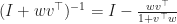
$(A+uv^\top)^{-1} = (I + wv^\top )^{-1} A^{-1} = \Big( I - \frac{wv^\top }{ 1 + v^\top w} \Big) A^{-1} = A^{-1} + \frac{ A^{-1} u v^\top A^{-1} }{ 1 + v^\top A^{-1} u }\, .$

as required. $\square$

The following in some sense repeatedly analyses to the determinant under the Sherman-Morrison formula.

Lemma 2. If $w_1 , w_2,...$ are a sequence of vectors and we let $A_n = \sum_{k=1}^n w^\top_k w_k$ then

$\sum_{k=p+1}^N w_k^\top A^{-1}_k w_k = \mathcal O ( \log \lambda_{\max}(A_n))\,.$

Proof. First note that if $A= B + w^\top w$ then, as was also in the Sherman-Morris formula

$| B | = | A - w^\top w | = | A | ( 1 - w^\top A^{-1} w)$

Thus

$w^\top A w = \frac{| A| - |B|}{|A|}$

which should remind you of the derivative of the logarithm. (Also note that this tells us that determinant is increasing and that $w^\top Aw \leq 1$ .) If we apply this to the above sum and apply the concavity of the logarithm

$\begin{aligned} \sum_{k=p+1}^N w_k^\top A^{-1}_k w_k = \sum_{k=p+1}^N \frac{|A_{k}|-|A_{k-1}|}{|A_{k}|} & \leq \sum_{k=p+1}^N \log |A_k| -\log |A_{k-1}| \\ & = \log |A_N| - \log |A_{p}| \end{aligned}$

Since $|A|$ is the product of all eigenvalues $\lambda_{\max}(n)^p \geq |A_N|$ . So we see that

$\sum_{k=p+1}^N w_k^\top A^{-1}_k w_k = \mathcal O( \log \lambda_{\max}(N))\, .$

$\square$

References

This is based on reading:

T.L Lai, Herbert Robbins, C.Z Wei, “Strong consistency of least squares estimates in multiple regression II”, Journal of Multivariate Analysis, Volume 9, Issue 3, 1979, Pages 343-361.

Lai, Tze Leung; Wei, Ching Zong. Least Squares Estimates in Stochastic Regression Models with Applications to Identification and Control of Dynamic Systems. Ann. Statist. 10 (1982), no. 1, 154–166. doi:10.1214/aos/1176345697.

Share this:

Like this:

Leave a Reply Cancel reply