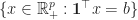
The Simplex Theorem suggests a method for solving linear programs . It is called the Simplex Algorithm.

Screen Shot 2018-05-30 at 07.03.39.png

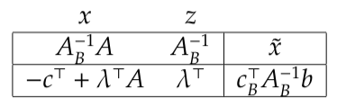
The tableau in Step 2 is called the Simplex Tableau. It stores all the information required in the Simplex Theorem: matrix $A$ expressed in terms of basis $B$ , $A^{-1}_BA$ ; the basic feasible solution excluding non-zero entries $A^{-1}_Bb$ ; the reduced cost vector $\tilde{c}^{\top}=c^{\top} - c_B^{\top} A^{-1}_B A$ , and the cost of the current solution $c_B^{\top} A^{-1}_Bb$ .
The bottom row of the simplex tableau is called the objective row.
Observe that the columns of the matrix $A^{-1}_BA$ corresponding to the basis $B$ necessary form an identity matrix. Note, by reading along the tableau, we can match each $1$ in this identity matrix to an entry of the column vector $A^{-1}_Bb$ . From this, we can recover the bfs given by basis $B$ , $x=(A^{-1}_Bb,0)$ .
The Simplex Algorithm also works for inequality constraints. For an optimization with inequality constraints $Ax\leq b$ , when we add slack variables $z\geq 0$ , we have equality constraints $Ax+Iz=b$ . Observe for new matrix $A'=(A\; I)$ , $(x,z)=(0,b)$ is a basic solution. Thus, provided $b>0$ , $(x,z)=(0,b)$ is a basic feasible solution.
In Step 3, we call $i$ the pivot row, $j$ the pivot column, and $(i,j)$ the pivot.

If Step 2 follows Step 3, we need to calculate $A^{-1}_{\tilde{B}}$ from $A^{-1}_{{B}}$ . In other words, we need to apply operation $A^{-1}_{\tilde{B}}A_B$ . We can break down Step 2 into the following routine

Screen Shot 2018-05-30 at 07.04.33.png

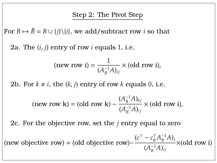
In other words, The matrix $A^{-1}_BA$ is exactly the matrix formed by multiplying and adding rows of $A$ so that the resulting matrix has an identity matrix in the columns corresponding to basis $B$ . The reduced cost vector $\tilde{c}^{\top}_B$ is exactly the vector formed by multiplying and adding rows of $A$ so that there are zeros in the components corresponding to basis $B$ . Because these identity matrix and zero components are necessary, you can always tell if your simplex tableau is in the correct form.

In addition, Step 3 can be expressed in terms of the Simplex Tableau in the following way.

Screen Shot 2018-05-30 at 07.05.22.png

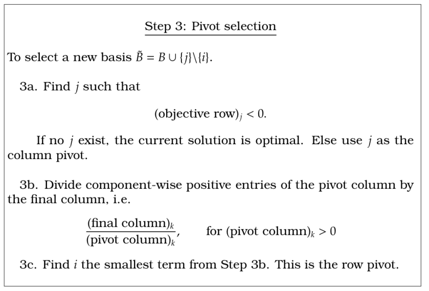
In Step 3a, we do not include the final entry of the objective row in our calculations.
In Step 3b, we do not include the entry $k$ , corresponding to the objective row, in our calculations.

Let’s now go through a simple example in detail.

Example 1. $\:$

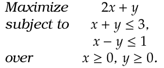
Screen Shot 2018-05-30 at 07.08.09.png Screen Shot 2018-05-30 at 07.12.17.png

Answer 1. This is the same as

Screen Shot 2018-05-30 at 07.08.17.png

Let’s go through the steps of the algorithm.

Step 1: we find a basis. As we noted inequality constraints mean we can start with all slack variables in the basis.

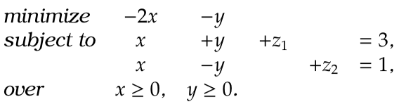
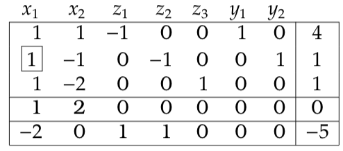
Step 2: write out the simplex tableau:

Screen Shot 2018-05-30 at 07.08.24.png

The basis variables, $z_1$ and $z_2$ , are starred and our current solution can be read from the final column: $(x,y,z_1,z_2)= (0,0,3,1)$ . As required, there is an identity matrix beneath the basis variables; as required, there are zeros beneath basis variables in the objective row. So the tableau is in the correct form.

Step 3: the reduced cost for both variables $x$ and $y$ are negative: $-2$ and $-1$ respectively. Thus, we could pivot on either column. We decide to pivot on $x$ . So, $x$ will be added to the basis. We need to remove a variable from the basis. We perform Step 3b.

Screen Shot 2018-05-30 at 07.08.31.png

The $x$ -row divided by the final row gives $3/1$ and $1/1$ . As $1$ is smallest we pivot on the second row. For book keeping, we place a box around the pivot. We now repeat to Step 2.

Step 2: For the matrix to be in the correct form, we must multiply and subtract the pivot row from all other rows so that the only non-zero entry in the pivot row is a $1$ at the pivot. In this case, the pivot row is in the correct form (the pivot contains a $1$ ), we deduce the pivot row from the 1st row, and we add two lots of the pivot row to the objective row. This gives a tableau

Screen Shot 2018-05-30 at 07.08.37.png

Step 3: The only negative reduced cost is for $y$ . This gives the pivot column. The only positive term from Step 3b is from the first row; this is our pivot row.

Screen Shot 2018-05-30 at 07.08.43.png

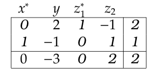
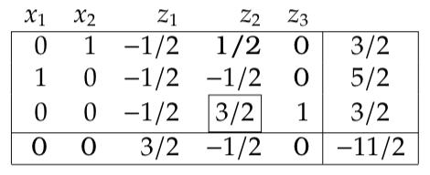
Step 2: dividing the pivot row by $2$ and adding that to the 2nd row and three times to the objective row gives

Screen Shot 2018-05-30 at 07.08.48.png

The reduced costs in the objective row are all positive. Thus, the current solution is optimal. Once again we read this solution from the simplex tableau by associating basis variables with the final column through the $1$ ’s in the identity submatrix. In particular, $x=2$ and $y=1$ and the value of the maximum is $5$ . $\square$

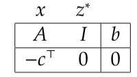
We can make more general observations from our example, for the following optimization:

Screen Shot 2018-05-30 at 07.12.17.png

Once slack variables are added to , these slack variables can form a basis with $A^{-1}_{B_z}=I$ .
If $b>0$ then $z=b$ , $x=0$ forms a basic feasible solution, and since our objective does not constrain slack variables, the following tableau forms a correctly initialized simplex tableau

Screen Shot 2018-05-30 at 07.12.53.png

Now considering this tableau again with respect to another basis, $B$ . Letting $\lambda^{\top}=c^{\top}_{B}A_{B}^{-1}$ and $\tilde{x}=A_{B}^{-1}b$ , we get

Screen Shot 2018-05-30 at 07.12.57.png

From the tableau above, once again $\tilde{x}$ gives the values of basic variables; we can also find our current inverse matrix $A_B^{-1}$ ; we can find our dual variables $\lambda^{\top}$ .
The Simplex Algorithm maintains primal feasibility $\tilde{x}\geq 0$ ; as any variable in the basis has a zero in the objective row, the Simplex Algorithm maintains complementary slackness $\lambda^{\top} z=0$ and $(c^{\top}-\lambda^{\top} A)x=0$ ; when the Simplex Algorithm is complete the objective row is positive, so we have dual feasibility $\lambda^{\top} A\geq c^{\top}$ and $\lambda^{\top}\geq 0$ .
In other words, whilst maintaining primal feasibility and complementary slackness, we search for dual feasibility. Once this is found by Linear Programming Lemma 2, our solution is optimal both for the primal and dual problem.

Two Phase Simplex

We consider the method of two stage simplex with the following example. $\label{FS:example} \text{Minimize}\quad x_1+2x_2\quad \text{ subject to }\quad x_1+x_2\geq 4,\quad x_1-x_2\geq 1,\quad -x_1+2x_2\geq -1\quad \text{over} \quad x_1\geq 0,\quad x_2\geq 0$ which, adding slack variables, is equivalent to this first problem

Screen Shot 2018-05-30 at 07.14.24.png

Observe that, unlike before, setting $(x_1,x_2)=(0,0)$ does not yield a basic feasible solution. In particular, if $x_1=x_2=0$ then $z_1=-4$ , $z_2=-1$ which are not feasible. So, we need to find a bfs to start from. The trick is to solve a different optimization problem whose optimal solution is a bfs for our original problem.

For example, we consider the second problem

Screen Shot 2018-05-30 at 07.14.54.png

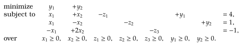
We added an extra variable $y$ to each constraint that was negative in our original problem. The positive variable $y=(y_1,y_2)$ tracts the amount we have violated any of our constraints.
We then chose to minimize $y_1+y_2$ which we interpret as the total amount that we have violated our constraints.
Note by adding these extra variables there is a bfs with $x_1=x_2=0$ , where $(y_1,y_2,z_3)=(4,1,1)$ . So, we can solve the second problem using the Simplex Algorithm.

Both problems have the same number of non-zero entries in a bfs, namely, $3$ . There is a feasible solution to the first problem iff the optimal value of the second problem is zero. Thus, once we have solved the second problem, we will be at a basic feasible solution, where $y_1=y_2=0$ . Removing variables $y_1$ and $y_2$ , this is then a basic feasible solution to the first problem: all the violated constraints are satisfied and there are the right number of non-zero terms. So we should solve this problem in two phases:

Phase I: Solve the second problem, where we added additional variables for violated constraints.

Phase II: Removing the additional variables we have a bfs for the first problem. We then solve the second problem.

So now we can solve this problem using the Simplex algorithm in two phases:

Phase I: Screen Shot 2018-05-30 at 07.15.42.png

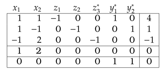
We have written down the simplex tableau for the second problem and added an additional objective row for the objective of the first problem. Notice the simplex tableau is not in the correct form. First, we want $z_3$ , $y_1$ and $y_2$ to be basis elements. So we need to multiply the 3rd row by $-1$ . Second, the Phase I objective row contains non-zero entries above basic feasible variables $y_1$ , $y_2$ . So we need to subtract the first and second rows of the simplex tableau from the bottom objective row.

Screen Shot 2018-05-30 at 07.16.05.png

We now proceed to optimize the this tableau whilst treating the additional objective row as though it was just an additional constraint.

Screen Shot 2018-05-30 at 07.16.30.png

We are now at an optimal solution for the the first phase. In particular, we are at a basic feasible solution where $x_1=5/2$ and $x_2=3/2$ . We can now remove $y_1$ and $y_2$ , the bottom row and solve the second phase.

Phase II:

Screen Shot 2018-05-30 at 07.17.25.png

Screen Shot 2018-05-30 at 07.17.52.png

So we have now solved our original optimization problem. The optimal solution is $x_1=3$ , $x_2=1$ with optimal value $5$ .

Dual Simplex

Dual simplex is another method for finding a basic feasible solution from a non-feasible basic solution. The Simplex Algorithm maintains feasibility of the primal problem; this is why we minimize ). The Simplex Algorithm searches for a solution that is dual feasible. The dual simplex takes a solution that is dual feasible and searches for a primal feasible solution.

We continue our example from the last section. Here we solved, . We now notice we forgot a constraints $3x_2\geq 4$ . So we want to solve

Screen Shot 2018-05-30 at 07.19.58.png

Our previous optimal simplex tableau was

Screen Shot 2018-05-30 at 07.20.28.png

But now notice, our current solution $x_1=3$ , $x_2=1$ is no longer feasible as $3x_2 < 4$ . We now wish to solve this problem by adding this constraint and its a slack variable to our tableau:

Screen Shot 2018-05-30 at 07.20.32.png

Multiplying the $4$ th row by $-1$ and then adding $3$ times the first row to the fourth puts the tableau in the correct form for our basis.

Screen Shot 2018-05-30 at 07.20.37.png

Our current basic solution has $z_4=-1$ . So our basis is not feasible for our primal problem ; however, the objective row suggests a dual feasible solution. Note below our slack variables in our , our tableau contained a negative identity matrix $-I$ , and $\lambda^\top=c_B^\top A^{-1}_B=(4/3,0,1/3,0)\geq 0$ and $c_B^\top - \lambda^\top A_B=0-\lambda^\top (-I) =(4/3,0,1/3,0)\geq 0$ .

We select a pivot on rows that maintains dual feasibility and increases our objective to a primal feasible solution i.e. $A^{-1}_B b\geq 0$ . We choose a row $i$ for which primal feasibility is violated i.e. $(A^{-1}_B)_i<0$ . In our example, this is the $4$ th row. We then divide the objective row with the negative entries from this row and find the least negative entries. In our example, the third column gives $(4/3)/-1= -4/3$ and the fifth column gives $(1/3) / -1= -1/3$ . So as $-4/3 > -1/3$ , we pivot on the fifth column. . This gives the tableau

Screen Shot 2018-05-30 at 07.22.18.png

Our current solution is feasible and, as our pivot kept our objective row positive, our solution is now optimal. In particular, $(x_1,x_2)=(8/3,4/3)$ .

Linear programming and simplex results

Theorem 1. The extreme points of $\mathcal X(b)=\{x: Ax=b, x\geq 0\}$ are exactly the set of basic feasible solutions.

Proof. Recall that we assume each $d\times d$ submatrix of $A$ is invertible. Thus for each basis, $B$ there is a unique basic feasible solution (bfs) $x=(x_B,0)$ . Take this $x$ and suppose $x=p x^1 + (1-p)x^2$ for some $x_1=(x_B^1,x^1_N), x_2=(x_B^2,x^2_N)\in \mathcal X(b)$ . If $x^1_N\neq 0$ then, because $px^1_N+(1-p)x^2_N=0$ , then either $x_i^1<0$ for some $i\in N$ or $x_i^2<0$ for some $i\in N$ , which contradicts the feasibility of $x^1$ and $x^2$ . If $x^1_N=0$ then $x^2_N=0$ and so by uniqueness of bfs $x$ , $x^1=x^2=x$ . Thus any bfs $x$ is an extreme point.

Conversely, take any feasible $x$ that is not a basic feasible solution. Let $D=\{ i : x_i>0\}$ and $M=\{ i : x_i=0\}$ as $x$ is not a basic feasible solution $D$ has more than $d$ points. So the submatrix $A_D$ has linearly dependent columns, i.e. there exists a $y=(y_D,0)\neq 0$ such that $Ay=A_Dy_D=0$ . Take $x^1=x+\delta y$ , $x^2=x-\delta y$ where $\delta$ is sufficiently small so that $x_D \pm \delta y_D >0$ . Since $Ax_1=Ax + \delta Ay=b+0=b$ , $x_1$ and $x_2$ are feasible and also $\frac{1}{2} x^1+\frac{1}{2} x^2 = x$ . So $x$ is not an extreme point. $\square$

Theorem 2. Any linear program with a finite optimum has at least one optimum at an extreme point.

Lemma 1. For a closed convex set $\mathcal C\subset \mathbb R^p$ , if $\mathcal H=\{ x : a^\top x=c\}$ is a separating hyperplane, i.e. $\mathcal C \subset \{ x : a^\top x\geq c\}$ , them an extreme point in $\mathcal H \cap \mathcal C$ is an extreme point in $\mathcal C$ .

Proof. Assume $x=px_1+ (1-p)x_2$ for $x_1,x_2\in\mathcal C$ for $p\in (0,1)$ . Then $c=a^\top x= p a^\top x_1 + (1-p) a^\top x_2$ . By assumption $a^\top x_1\geq c$ and $a^\top x_2\geq c$ . So, $a^\top x_1= c$ and $a^\top x_2= c$ . Thus $x_1,x_2\in\mathcal H\cap\mathcal C$ but $x$ is an extreme point in $\mathcal H\cap \mathcal C$ so $x=x_1=x_2$ . So $x$ is an extreme point in $\mathcal C$ . $\square$

Theorem 3 [Carathéodory’s Theorem] Every closed bounded convex set $\mathcal C\subset \mathbb R^d$ has an extreme point and every point in $\mathcal C$ is a convex combination of its extreme points. Moreover, the number of extreme points required in this convex combination can be chosen to be less than or equal to $d+1$ .

Proof. We prove the result by induction on $d$ . For $d=1$ , $\mathcal C$ is a closed bounded interval and the extreme points are the end points of the interval. Assuming the result holds for dimensions less than $d$ , we prove the result for $d$ . Firstly, note if $\mathcal C$ has empty interior then $\mathcal C$ is a subset of an affine space, $\mathcal A=\{ \lambda x_1 + (1-\lambda) x_2: x_1,x_2\in\mathcal C, \lambda\in\mathbb R\}$ and this space must have dimension of $d-1$ or less otherwise $\mathcal C$ would have a non-empty interior. In otherwords, if $\mathcal C^\circ=\emptyset$ , then problem is immediately reduced to the $d-1$ dimensional case.

Take $x\in\mathcal C$ if $x$ is an extreme point then everything is trivial. So let’s suppose $x$ is not an extreme point, in which case there exist an $x_1,x_2\in\mathcal C$ and $p\in (0,1)$ such that $x=px_1+(1-p)x_2$ and $x_1\neq x_2$ . Consider the line $x(\lambda)=\lambda x_1 + (1-\lambda)x_2$ , for $\lambda\in\mathbb R$ . Let $y_1=x(\lambda_1)$ where $\lambda_1$ is the largest $\lambda$ such that $x(\lambda)\in\mathcal C$ and let $y_2=x(\lambda_2)$ where $\lambda_2$ is the smallest $\lambda$ such that $x(\lambda)\in\mathcal C$ . Note $y_1$ and $y_2$ are well defined because $\mathcal C$ is closed and bounded. It is also clear that $x=q y_1 + (1-q)y_2$ for some $q\in (0,1)$ and $y_1,y_2\notin \mathcal C^\circ$ . Thus the applies to $y_1$ and $y_2$ . Let $\mathcal H_1$ and $\mathcal H_2$ be the hyperplanes respectively sepaarating $y_1$ and $y_2$ from $\mathcal C$ . Then $\mathcal H_1\cap \mathcal C$ and $\mathcal H_2\cap \mathcal C$ convex sets of dimension less than $d-1$ . Thus by the induction hypothesis both $y_1$ and $y_2$ are a convex combination of the extreme points which exist in $\mathcal H_1\cap \mathcal C$ and $\mathcal H_2\cap \mathcal C$ respectively, which by Lemma 1 are extreme points of $\mathcal C$ . So,as $x$ is a convex combination of $y_1$ and $y_2$ , $x$ is a convex combination of extreme points existing in $\mathcal C$ .

Now, we reduce the number of extreme points required to express $x$ . Suppose $x=\sum_{i=1}^n p^i x^i$ , where $\sum_{i=1}^n p^i =1$ , $p_i>0$ and where each $x_i$ is an extreme point. If $n > d+1$ then the vectors $x^1-x^n, x^2- x^n,...,x^{n-1}- x^n$ are linearly dependent. Thus there exists $(q^1,...,q^{n-1})\neq 0$ where, defining $q_n=-\sum_{i=1}^n q^i$ , we have $\sum_{i=1}^{n} q^i x^i = \sum_{i=1}^{n-1} q^i (x^i -x^n)=0$ . Notice because $(q^1,...,q^{n-1})\neq 0$ and because by definition $\sum_{i=1}^n q^i=0$ , there must exist some $q^i>0$ We, now, consider $\sum_{i=1}^n (p^i - t q^i)x^i$ . If we take $t=\max_i \{p^i/q^i : q^i>0 \}$ , then any $i$ maximizing this expression is zero in the sum $\sum_{i=1}^n (p^i - t q^i)x^i$ . In otherwords, $x$ in now the convex combination of less than $n-1$ extreme points. Continuing inductively, we find $x$ can be expressed as the convex combination of $d+1$ points or less. $\square$

Proof of Theorem 2. Let $x^*$ be the finite optimum to a linear program with objective $c^\top x$ and feasible set given by polytope $\mathcal C\subset \mathbb R_+^p$ . So for hyperplane $\mathcal H=\{ y : c^\top y =c^\top x^*\}$ , $\mathcal H\cap \mathcal C$ defines a non-empty polytope of optimal solutions. We aim to apply Caratheodory’s Theorem. Since $\mathcal C\subset \mathbb R_+^p$ , for $\mathbf{1}^\top x \geq 0$ for all $x\in\mathcal C$ . Also note $\{x\in\mathbb R_+^p: \mathbf{1}^\top x=b\}$ is closed and bounded for all $b\geq 0$ . Thus $b$ , the minimum $\mathbf{1}^\top x$ over $x\in \mathcal H\cap \mathcal C$ , is well defined and attained. Thus, as $\mathcal H'=\{ x\in \mathbb R_+^p: \mathbf{1} x=b\}$ is a closed bounded set and so $\mathcal H'\cap\mathcal H \cap \mathcal C$ is a closed bounded non-empty polytope of optimal solutions, which by Caratheordory’s Theorem must contain an extreme point. Applying Theorem 1 twice – once for $\mathcal H$ and once for $\mathcal H'$ – this optimal point must be an extreme point in $\mathcal C$ also. $\square$

In this definition direction of an arc does not matter. This will soon make sense.↩
When $M_{ij}<\infty$ for some $(i,j)$ , these comments hold for the enlarged matrix with slack variables appropriately added.↩
Our tree solution is different because our feasible solution is different.↩