Linear Programming

A linear program is a constrained optimization problem with a linear objective, $f(x):=c^\top x$ , and linear functional constraints, $h(x):=Ax$ , we could for instance write

Screen Shot 2018-05-30 at 06.34.56.png

Here $c\in{\mathbb R}^p$ is a vector, $A$ is an $d\times p$ matrix with row vectors $A_j$ and, as before, $b\in{\mathbb R}^d$ and $x\in{\mathbb R}^p$ and $d\leq p$ .
A linear program could have some equality constraints $A_jx = b_j$ or could optimize some variables over $x_i$ over ${\mathbb R}$ . Even so, with the addition of extra variables, constraints and suitable choice of $c$ , $A$ and $b$ , the above optimization can express any linear program.
There are various ways to interpret . To start with, we could interpret $c^\top=(c_1,..,c_p)$ as the running cost of $p$ different machines types. The vector $b^\top=(b_1,..,b_d)$ could represent the required rate of production of $d$ different goods. If a matching $i$ makes good $j$ at rate $a_{ij}$ , the $ij$ component of $A$ , then a constraint $A_j x \geq b_j$ must be met and the optimization asks to minimize the cost of production subject to the production constraints.
Because our objective and constraints are convex, we can apply the Lagrangian approach.

Lemma 1. The dual of is the optimization

$\label{LP:D}\tag{Dgeq} \maxi\quad b^\top y \quad \text{subject to} \quad A^\top y \leq c\quad \text{over} \quad y\geq 0.$

Proof. Including slack variables $z\in{\mathbb R}_+^p$ , we minimize the Lagrangian with Lagrange multipliers $y\in{\mathbb R}^d$

$\begin{aligned} \min_{x\geq 0, z\geq 0} c^\top x +y^\top(b+z-Ax) & = \min_{x\geq 0, z\geq 0} y^\top b +y^\top z+ (c^\top-y^\top A)x \\ & = \begin{cases} y^\top b & \text{if } c^\top \geq y^\top A\text{ and } y\geq 0\\ -\infty & \text{otherwise}. \end{cases} \end{aligned}$

So by maximizing, the dual of is as required: $\max \;\; b^\top y\;\text{subject to}\; A^\top y \leq c\; \text{over}\; y\geq 0.$ $\square$

Lemma 2. If $x$ is feasible for and $y$ is feasible for and they obey the complementary slackness conditions $y^{\top}(b-A x)=0$ and $x^T(c-A^\top y)=0$ then $x$ is optimal for and $y$ is optimal for .

Proof. By Weak Duality, for all primal feasible $x$ and dual feasible $y$ , $c^\top x \geq b^\top y$ . But for $x$ and $y$ as above, $c^\top x= c^\top x + y^\top( b-Ax) = b^\top y + x^\top(c-A^\top y) = b^\top y$ . Thus we see the primal and dual are equal and thus these $x$ and $y$ are optimal. $\square$

The set ${\mathcal X}(b):=\{ x\geq 0 : Ax \geq b \}$ is the intersection of $d$ half-spaces. In other words, the feasible set is a convex polytope.

An extreme point point of a convex polytope ${\mathcal X}(b)$ (or indeed any convex set) is a point $x\in{\mathcal X}(b)$ such that if $qy+(1-q)z=x$ for some $y,z\in{\mathcal X}(b)$ $q\in (0,1)$ then $x=y=z$ .
For a polytope we think of an extreme point as a point on the corner of the shape.

Theorem 1. Any linear program with a finite optimum has at least one optimum at an extreme point.

So, we just need to check extreme points to find an optimum. Let’s consider the optimization

Screen Shot 2018-05-30 at 06.35.48.png which, as we know, can be made equivalent to .

Consider $d\times p$ matrix $A$ and let $B\subset \{1,...,p\}$ where $|B|=d$ . We let $A_B$ be the $d\times d$ submatrix of $A$ formed by removing the columns not in $B$ . We call the matrix $A_B$ a basis.¹ Given $A$ and $B$ , we use the notation $N=\{1,...,p\}\backslash B$ , $x=(x_B,x_N)$ and

where here elements are understood to be ordered relative to $B$ and $N$ . If $x=(x_B,x_N)=(x_B,0)$ , i.e. non-basis elements are zero, and $A_Bx_B=b$ then we call $x$ a basic solution. We call a positive basic solution a basic feasible solution (bfs).

Henceforth, we make the following assumptions on the matrix $A$ and vector $b$ .

Assumption 1. The rows of $A$ are linearly independent.

Assumption 2. Every basic solution $x=(x_B,0)$ has exactly $d$ non-zero variables.

Assumption 3. Every $d\times d$ submatrix of $A$ is non-singular.

Assumption 1 removes redundant constraints from optimization .
Assumption 3 implies that the rows of basis $A_B$ are a basis of vector space ${\mathbb R}^d$ .
Assumptions 2 and 3 can be made to hold by an infinitesimally small perturbation of the entries of $A$ .
Assumptions 2 and 3 imply that each basis $B$ uniquely specifies a bfs $x=(A^{-1}_Bb,0)$ .

The extreme points for the feasible set of $\eqref{LP:Opt=}$ can be found.

Theorem 2. The extreme points of ${\mathcal X}(b)=\{x: Ax=b, x\geq 0\}$ are exactly the set of basic feasible solutions.

Finding a extreme point is now characterized and computable, namely, we find $x=(x_B,0)\geq 0$ where $x_B=A^{-1}_B b$ .

Theorem 3. [Simplex Theorem] Given Assumptions 1–3, for , a basic feasible solution $x=(A^{-1}_Bb,0)$ is optimal iff

$\label{LP:OptCond} 0\leq c_N^\top-c_B^TA^{-1}_B A_N$

Moreover, if $x$ is not optimal, i.e. $0>(c_N^\top-c_B^TA^{-1}_B A_N)_j$ for some $j\in N$ , then there exists a new basis $\tilde{B}=B\cup \{j\} \backslash \{i\}$ for some $i\in B$ such that the basic feasible solution $\tilde{x}=(A^{-1}_{\tilde{B}},0)$ satisfies $c^\top \tilde{x} < c^\top x$ .

This theorem gives both a method to verify optimality of a bfs and a mechanism to move to a better bfs from a non-optimal bfs. As we will discuss, this method is called the Simplex Algorithm.
For a maximization, the inequality in is reversed.
Since $c^\top_B-c_B^\top A^{-1}_B A_B =0$ , optimality condition can be expressed as

$\label{LP:OptCondII} 0\leq c^\top-c_B^\top A^{-1}_B A =:\tilde{c}^\top.$

The vector $\tilde{c}$ , defined above, is called the reduced cost vector and its entries are reduced costs.
We can interpret $\lambda^\top=c_B^TA^{-1}_B$ as variables of the dual of . So once $\tilde{c}=c^\top-\lambda^\top A\geq 0$ , we have a dual feasible solution $\lambda$ and a primal feasible solution $x=(A^{-1}_Bb,0)\geq 0$ . Thus, by essentially the same argument we used in Lemma [LP:primaldualcomp], both $x$ and $\lambda$ are optimal for the primal and the dual problems respectively.

Proof of the Simplex Theorem. Let’s compare bfs $x=(A_B^{-1}b,0)$ to a feasible solution $y=(y_B,y_N)$ . As $y$ is feasible $A_B y_B + A_Ny_N=b$ . Thus, using Assumption 3,

$\label{LP:yB} y_B =A^{-1}_B b - A_B^{-1} A_N y_N.$ So

$\begin{aligned} \quad c^\top x \leq c^\top y \:\: & \iff\:\: c^\top_B A_B^{-1} b \leq c_B^{\top}( A_B^{-1}b -A_B^{-1}A_N y_N ) + c_N^\top y_N \:\: \\ & \iff \:\: 0\leq (c_N^\top - c^\top_B A_B^{-1}A_N )y_N. \end{aligned}$

Thus, if holds then the bfs $x$ is optimal. Conversely, by Assumptions 2 and 3, for any $y_N$ sufficiently small, i.e. $\forall y_N>0$ s.t. $|y_N|\leq \delta$ for some $\delta>0$ , we can choose $y_B$ so that $y=(y_B,y_N)$ is feasible. Namely, $y_B$ is given by , and it is positive because it is close to $x_B$ . Hence

$\begin{aligned} & c^\top x\leq c^\top y,\quad\forall y\in {\mathcal X}(b) \\ \implies & 0 \leq (c_N^\top - c^\top_BA_B^{-1}A_N )y_N,\quad \forall y_N\geq 0\:\; s.t. \;\; |y_N|\leq \delta \\ \implies & 0\leq c_N^\top -c^\top_BA_B^{-1}A_N. \end{aligned}$

This verifies that is necessary and sufficient for optimality.

Now suppose that bfs $x$ is not optimal, i.e. $0>(c_N^\top - c^{\top}_BA_B^{-1}A_N)_j$ for some $j\in N$ . This suggests we should increase the $j$ -th component. Take $x(t)=(A_B^{-1}b,0)+t(-A_B^{-1}A_Ne_j,e_j)$ where $e_j$ is the $j$ th unit vector in ${\mathbb R}^N_+$ and $t>0$ . Note

Screen Shot 2018-05-30 at 06.37.58.png

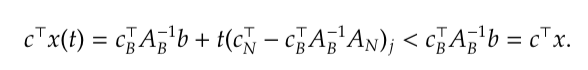
So the larger $t$ is the more $c^{\top} x(t)$ improves on $c^{\top} x$ . The biggest $\tilde{t}$ so that $x(\tilde{t})$ is feasible is

$\label{LP:topt} \tilde{t} = \min_{i\in B} \bigg\{ \frac{(A_B^{-1}b)_i}{(A_B^{-1}A_N)_{ij}} : (A_B^{-1}A_N)_{ij}>0\bigg\}$

Observe, if no such $\tilde{t}$ exists then $c^{\top} x(t)$ is unbounded. Otherwise, take $i$ to be the argument minimizing . Note $x(\tilde{t})$ is a bfs on $\tilde{B}=B\cup \{j\} \backslash \{i\}$ with $c^{\top} \tilde{x} < c^{\top} x$ . $\square$

When $A$ is known, we can use the term “basis” interchangeably to mean $B$ or $A_B$ .↩

3 thoughts on “Linear Programming”

Naren Sundar says:

May 31, 2018 at 3:53 am

Thanks! Could you give me a good link that introduces this business of this ‘dual’ concept in optimization? I often see it but I don’t understand how it comes about or what it is.

LikeLike

1. appliedprobability says:
  
  May 31, 2018 at 4:42 am
  
  Hi Naren,
  I’ve updated the post on Lagrangian Optimization. If you read everything up to Theorem 2 on that post. You should have everything you need.
  
  LikeLike
  
  1. Naren Sundar says:
    
    May 31, 2018 at 1:37 pm
    
    Thank you!
    
    LikeLike