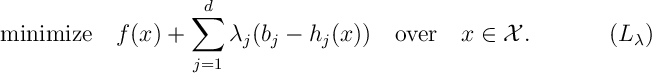
We are interested in solving the constrained optimization problem

The variables $x$ must belong to the constraint region ${\mathcal X}$ , where ${\mathcal X}$ is a subset of ${\mathbb R}^p$ .
The variables must satisfy the functional constraints $h(x)=b$ , where $latex h:{\mathcal X}\rightarrow{\mathbb R}^d$ and $b\in{\mathbb R}^d$ .
Variables that belong to the constraint region and satisfy the functional constraints are called feasible and belong to the feasible set

The variables are judged according to the relative magnitude of the objective function $f:{\mathcal X}\rightarrow{\mathbb R}$ .
A feasible solution to the optimization, $x^*$ , is called optimal when $f(x^*)\leq f(x)$ for all $x\in{\mathcal X}(b)$ .
In general, an optimum $x^*$ need not exist.
Inequality constraints $h_j(x)\leq b_j$ can be rewritten as equality constraints $h_j(x)+z_j=b_j$ , where $z_j\geq 0$ . Then an optimization of the form can be solved over variables $(x,z)\in{\mathcal X}\times{\mathbb R}_+^{p'}$ . The variables $z$ are called slack variables.
$\max_{x\in{\mathcal X}(b)} f(x) = - \min_{x\in{\mathcal X}(b)} -f(x)$ , so maximizing is the same as minimizing.

The set ${\mathcal X}$ could incorporate the functional constraints $\{x:h(x)=b\}$ , but generally we assume ${\mathcal X}$ is a set where the unconstrained optimization, $\min_{x\in{\mathcal X}} f(x)$ , is easier to solve. For example, ${\mathcal X}$ might be ${\mathbb R}_+^p$ and $\min_{x\in{\mathcal X}} f(x)$ might be solved by differentiating and finding local minima. What makes the problem difficult is the functional constraints. To get some solution, we might penalize going over these constraints. If so, we could remove these constraints and solve a different optimization

In the above optimization, the objective function

is called the Lagrangian of the optimization problem .

We call the components of the vector, $\lambda\in{\mathbb R}^d$ , Lagrange multipliers.
We use $x^*(\lambda)$ to notate its optimum of , if it exists.
For each inequality constraint $h_j(x)\leq b_j$ , a variable $z_j\geq 0$ is added and the term $\lambda_j(b_j-h_j(x))$ is replaced by $\lambda_j(b_j-z_j-h_j(x))$ . Because we introduced a new term $-\lambda_jz_j$ , for a finite solution to , we require $\lambda_j\leq 0$ and thus, after minimizing over $z_j$ , we have $z^*_j\lambda_j=0$ . This equality is called complementary slackness.
If $(x^*,z^*)$ our optimal Lagrangian solution is also feasible then complementary slackness states $\lambda_j( b_j- h_j(x^*))=0.$

The unconstrained optimization is, in principle, much easier to solve and a good choice of $\lambda$ can be used to penalize constraints that are not satisfied. For example, if we solve the optimization problem with optimum $x^*(\lambda)$ and found that $b_i>h(x_i)$ then, intuitively, we would make $\lambda_i$ bigger in order to make the price of overrunning constraint $i$ higher. Hopefully, this would then make the solution of closer to . The minimum of the Lagrangian is always smaller.

Lemma [Weak Duality] For all $\lambda\in{\mathbb R}^d$

Proof

$\square$

In fact, if we can make the two solutions equal then we have optimality.

Theorem 1 [Lagrangian Sufficiency Theorem] If there exists Lagrange multipliers $\lambda^*$ and a solution $x^*(\lambda^*)$ to $(L_{\lambda^*})$ such that $x^*(\lambda^*)$ is feasible for then $x^*(\lambda^*)$ solves the optimization problem (P).

Proof As $x^*(\lambda^*)$ is feasible then certainly $f(x^*(\lambda^*))\geq \min_{x\in{\mathcal X}(b)} f(x)$ . Now,

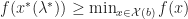
$f(x^*(\lambda^*))= f(x^*(\lambda^*)) + \lambda^{*T}(b-h(x^*(\lambda^*)))\tag{as $x^*(\lambda^*)$ is feasible}$

$= \min_{x\in{\mathcal X}} L(x;\lambda^*)\tag{as $x^*$ is optimal for $(L_{\lambda^*})$}$

So, $f(x^*(\lambda^*))= \min_{x\in{\mathcal X}(b)} f(x)$ .

$\square$

This result gives a simple procedure to solve an optimization:

Take your optimization and, if necessary, add slack variables to make all inequality constraints equalities.
Write out the Lagrangian and solve optimization for $x^*(\lambda)$ .
By solving the constraints $h(x^*(\lambda))=b$ over $\lambda$ , find a $\lambda^*$ so that $x^*=x^*(\lambda^*)$ is feasible.By Lagrangian Sufficiency Theorem, $x^*$ is optimal.

Duality

Since weak duality holds, we want $\lambda$ to make the minimized Lagrangian as big as possible. Only then can a feasible Lagrangian optimum be found to solve the optimization . Thus we consider the following optimization,

Screen Shot 2018-05-31 at 05.23.54.png

Here $g(\lambda)=\inf_{x\in\mathcal X} L(x;\lambda)$ and $\Lambda=\{ \lambda : \inf_{x\in\mathcal X} L(x;\lambda)>-\infty \}$ .
We call this optimization problem the dual optimization and, in turn, we call the primal optimization.
Making dependence on $b$ explicit, use $\rho(b)$ to denote the optimal value of the primal problem and $\delta(b)$ to denote the optimal value of the dual. By weak duality $\delta(b)\leq \rho(b)$ . If $\delta(b)=\rho(b)$ then we say strong duality holds.
Observe, $\max_{\lambda} L(x;\lambda)= f(x)$ , if $h(x)=b$ and $\max_{\lambda} L(x;\lambda)= \infty$ , otherwise. So, $\rho(b)=\min_{x\in\mathcal X}\max_{\lambda} L(x;\lambda)$ and by definition $\delta(b)=\max_{\lambda} \min_{x\in\mathcal X} L(x;\lambda)$ . So strong duality corresponds exactly to the saddle point condition that

$\label{LO:saddlepoint} \min_{x\in\mX}\max_{\lambda} L(x;\lambda)=\max_{\lambda} \min_{x\in\mX} L(x;\lambda)$

Essentially, the Lagrangian approach will only be effective when we can find a 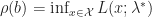$\lambda^*$ such that $\rho(b)=\inf_{x\in\mathcal X} L(x;\lambda^*)$ . This is equivalent to the existence of a supporting hyperplane for $\rho(b)$ .

Theorem 2. $\rho(b)=\inf_{x\in\mathcal X} L(x;\lambda^*)$ iff $\lambda^*$ and $\rho$ , together satisfy the property $\label{LO:Hyperplane} \rho(c) \geq \rho(b) + \lambda^{*\T}(c-b),\qquad\text{ for all }c\in\bR^d.$

Proof.

$\begin{aligned} \inf_{x\in\mX} L(x,\lambda) &= \inf_{x\in\mX}\Big\{ f(x) + \lambda^\T(b-h(x))\Big\} \\ & = \inf_{c\in\bR^d} \inf_{x\in\mX(c)} \Big\{ f(x) + \lambda^\T(b-h(x))\Big\} \\ & = \inf_{c\in\bR^d} \big\{ \rho(c) + \lambda^\T (b-c) \big\}.\end{aligned}$

So $\rho(b)=\inf_{x\in\mathcal X} L(x;\lambda^*)$ iff $\rho(b)=\inf_{c\in\mathbb R^d} \big\{ \rho(c) + \lambda^{*\T} (b-c) \big\}$ iff $\rho(b)\leq \rho(c) + \lambda^{*\T} (b-c)$ for all $c$ , as required.

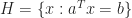
Informally, states that there exists a tangent to $\rho$ at point $b$ and that the function $\rho$ lies above this tangent.
The set $H=\{ (c,\rho(b) + \lambda^{*\T}(c-b))\in\mathbb R^{p+1}: c\in\mathbb R^d \}$ defines a hyperplane containing $(b,\rho(b))$ and $\{(c,\rho(c):c\in\mathbb R^d\}$ lies in the half-space above $H$ . So we call this “tangent” $H$ a supporting hyperplane to $\rho(b)$ at $b$ with slope $\lambda^*$ .
Any function $\rho:\mathbb R^d\rightarrow (-\infty,\infty]$ is convex if $q\rho(b)+(1-q)\rho(c) \geq \rho(qb+(1-q)c)$ , for $q\in [0,1]$ . It can be verified that this is equivalent to the condition . Optimization of convex functions may be possible with Lagrangian methods.
We discuss the relationship between convexity, hyperplanes, duality and Lagrangian optimization in the supplementary section, Section [DHLO].

Given , for $h>0$ , we can say that

$\frac{\rho(b+he_i)-\rho(b)}{h} \geq \lambda^*_i,\qquad \frac{\rho(b-he_i)-\rho(b)}{h} \leq \lambda_i^*.$

Thus, if $\rho$ is differentiable at $b$ then

$\label{LO:shadow} \frac{\partial \rho}{\partial b_i}(b)=\lambda^*_i.$

For a maximization problem, if we interpreted $\rho(b)$ as the optimal profit (or cost for a minimization problem) made when manufacturing using $b$ units of raw material then can be interpreted as the change in profit made from gaining a small additional quantity of material $i$ and thus $\lambda_i^*$ is interpreted at the price the manufacturer is prepared to pay to secure those extra goods.
From this interpretation, we call the optimal Lagrange multiplier $\lambda^*_i$ a shadow price.

As noted above if $\rho(b)$ is convex then we can find a $\lambda^*$ with which we can apply the Lagrangian approach.

For a constrained optimization problem we say Slater’s Condition is satisfied if the objective function $f$ is a convex function, if constraint region $\mathcal X$ is a convex set, if for each equality constraint $h_j(x)=b_j$ the function $h_j$ is linear, if there exist a feasible solution $x\in\mathcal X(b)$ such that all inequality constraint are satisfied with strict inequality $h_j(x)< b_j$ .
To make life easier we assume the functions $f$ and $h_j$ are continuous at the feasible $x$ assumed in slater’s condition and we assume there exists some non-optimal feasible solution in $\mathcal X(b)$ .

Theorem 3. If Slater’s Condition holds then $\rho(b)$ is a convex function and thus there exists $\lambda^*$ such that $\rho(b)=\inf_{x\in\mathcal X} L(x;\lambda^*)$ .

To prove this we will require the following (intuitively true) result.

Theorem 4. [Supporting Hyperplane Theorem] If $C$ is a convex set with non-empty interior and $z\notin C^\circ$ then there exist a supporting hyperplane $H$ that is a set $H=\{ x : a^T x=b \}$ with $z\in H$ and $C$ belonging a closed half-space associated with $H$ (i.e. $\{ x : a^T x\leq b \}$ or $\{ x : a^T x\geq b \}$ .

We can prove this result later, we will prove Theorem 3.

Proof of Theorem 3. By Slater’s condition the equality constraints are given by a matrix $H$ , i.e. $(Hx)_j=b_j$ for $j=1,...,d'$ . We assume that the image of $H$ has dimension $d'$ , otherwise, as row rank $=$ column rank for matricies, we can remove a redundant constraint.¹ Consider the set

$C= \{ ({b}',\rho)\in \bR^d\times \bR :\text{ there exists $x$ in feasible set $\mX({b}')$ with $f(x)\leq \rho$} \}$

So, roughly speaking, $C$ is all the stuff above $\rho(b')$ for each $b'$ .

We show that $C$ is convex. For $p\in (0,1)$ , $(b^1,\rho^1),(b^2,\rho^2)\in C$ and $x^1,x^2$ corresponding feasible points used in the definition of $C$ above, consider $(b^p,\rho^p)= p(b^1,\rho^1)+ (1-p) (b^2,\rho^2)$ and $x^p=px^1+(1-p)x^2$

Screen Shot 2018-05-31 at 05.27.44.png

The three statements above show that $(b^p,\rho^p)$ belongs to $C$ . So $C$ is convex.

Take $(b,\rho(b))$ . As $(b,\rho(b))\notin C^\circ$ , by the Supporting Hyperplane Theorem there exists a $(-\lambda,\mu)\in \mathbb R^d\times \mathbb R$ such

$-\lambda^\T c + \rho \mu \geq -\lambda^\T b + \rho(b) \mu$

Provided we can choose $\mu$ to be strictly positive then $\rho(c)$ has a supporting hyperplane in the sense of Theorem [LO:OptSHP] and so we are done. It is clear $\mu$ is positive: if we take $c=b$ and $\rho=f(x)$ for some non-optimal $x\in\mathcal X(b)$ the above inequality reads $\mu f(x) \geq \mu \rho(b)$ for all $x\in\mathcal X(b)$ , which is only true if $\mu \geq 0$ .

Now we show $\mu\neq 0$ . Let’s look for a contradiction: if $\mu=0$ then the supposting hyperplane would be vertical with respect to the component $\rho$ and we would have $c^\T \lambda \geq b^\T \lambda$ . Now applying Slater’s condition, there is a point $x$ where the inequality constraints are strict. By continuity of our inequality constraint function and by continuity of linear map $H$ for any $\delta$ suitably small we can choose $x(\delta)$ (close to $x$ ) such that

$h_j(x(\delta)) < b_j - \delta \lambda_j \quad\text{and} \quad (H x(\delta))_j = b_j - \delta \lambda_j.$

By continuity of $f$ we can choose $x(\delta)$ so that $f(x(\delta))<\infty$ . Thus, it is clear that $(b - \delta \lambda, f(x(\delta)) \in C$ but $\lambda^\T (b - \delta \lambda) < \lambda^\T b$ , which contradicts the earlier assertion that thus $\mu>0$ . Thus by taking $\lambda^* = (\lambda_j/\mu: j=1,...,d)$ we have