Sequential Monte Carlo (SMC)

Sequential Monte-Carlo is a general method of sampling from a sequence of probability distributions $\hat \eta_1,...,\hat \eta_t$ .

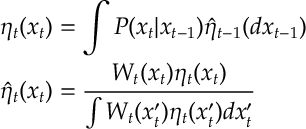
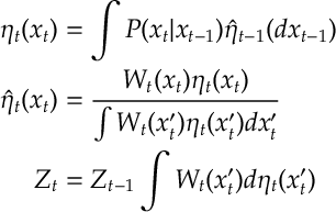
Here, we have the update equations

$\begin{aligned} \eta_t(x_t ) & = \int P(x_t | x_{t-1} ) \hat \eta_{t-1}(dx_{t-1}) \\ \hat \eta_t(x_t) & = \frac{W_t(x_t) \eta_t(x_t) }{ \int W_t(x'_t) \eta_t(x'_t) dx'_t }\end{aligned}$

Notice if we take $W_t(x) =\hat \eta_t(x)/\eta_t(x)$ then any sequence of distributions $\hat \eta_1,...,\hat \eta_t$ can be realized by the above recursion.¹ Except special cases, we cannot calculate the integrals above when the state space $\mathcal X$ is infinite (or simply large).

However, we can approximately sample from the required distribution and use that as a proxy. We can then update with the same equations as above replacing the continuous $\eta_t$ with the discrete $\eta^N_t$ which is achieved by taking $N$ samples. This is called Sequential Monte-Carlo (SMC).

More precisely, SMC does the following:

1) Resample. For $i=1,...,N$ $\begin{aligned} x^i_t \sim \hat \eta^N_t, \quad \hat x^i_{t+1} \sim P(\cdot | x^i_t ) \, .\end{aligned}$

2) Reweight.

$\begin{aligned} \hat \eta_{t+1}^N (x) := \sum_{i=1}^N \frac{W_{t+1}(\hat x_{t+1}^i)}{ W^\Sigma_{t+1} } \delta_{\hat x_{t+1}^i}(x)\, ,\end{aligned}$

where

$\begin{aligned} W_{t+1}(\hat x_{t+1}^i) = \frac{\hat \eta_{t+1} (\hat x_{t+1}^i)}{ \eta_t(\hat x_{t+1}^i)} \quad\text{and}\quad W^\Sigma_{t+1} = \sum_{j=1}^N W_{t+1}(\hat x_{t+1}^j) \, .\end{aligned}$

It is worth noting that the resampled RVs $x^i_t$ from the distribution $\hat \eta_t$ and thus are a random subset of $\{\hat x^i_t : i=1,..,N\}$ . Since we then apply transitions $P(\hat x|x)$ we should, in general, recover $N$ distinct points. We assume that it is easy to sample from $\hat \eta_1$ . Further notice, the algorithm is always dealing in ratios of the distributions $\eta_t$ . Thus we do not have to specify normalizing constants for these distributions if we do not know them (which is often the case in the world of Bayesian statistics). A final important point, is that although we assume $\hat x^i_t$ to be a state in the set $\mathcal X$ . We could allow it to be the set of previous states $\hat{x}^i_t = ( \hat{x}^i_s : s\leq t)$ . This is what we do in the hidden Markov models (discussed below).

Roughly why this works. Although we can say more precisely why things work out for this algorithm, let’s sketch out why it works. Suppose that $\eta_t^N$ is a good approximation of $\eta_t$ . So much so that we assume that $\eta^N_t=\eta_t$ (and thus $W_t(x) \propto \eta_t(x)$ ). Notice that from infinitely many resamples from $\hat \eta_t$ and $P$ gives:

$\begin{aligned} \label{SMC:just} \mathbb E_{\hat x \sim \hat \eta^N_{t+1}} \left[ f(\hat x) \right] = \frac{\sum_{i=1}^N f({\hat x_{t+1}^i})W_{t+1}({\hat x_{t+1}^i})}{\sum_{j=1}^N W_{t+1}({\hat x_{t+1}^j})} \, .\end{aligned}$

We can apply the strong law of large numbers to each of the two sums above. Notice that

$\begin{aligned} \lim_{N\rightarrow\infty} \frac{1}{N} \sum_{i=1}^N f({\hat x_{t+1}^i})W_{t+1}({\hat x_{t+1}^i}) & = \int f(\hat x) W_{t+1}(\hat x) P(\hat x| x) \hat \eta_t(x) dx d\hat x \\ & = \int f(\hat x) \left[ \frac{\hat \eta_{t+1} (\hat x)}{\eta_t(\hat x)} \right] P(\hat x| x) \hat \eta_t(x) dx d\hat x \\ & = \int f(\hat x) \hat \eta_{t+1}(\hat x) d\hat x \, .\end{aligned}$

This holds for $f$ and $f\equiv 1$ . Thus applying to , we see that

$\begin{aligned} \lim_{N\rightarrow\infty} \mathbb E_{\hat x \sim \hat \eta^N_{t+1}} \left[ f(\hat x) \right] = \int f(\hat x) \hat \eta_{t+1}(\hat x) d\hat x \, .\end{aligned}$

Thus we see that in the limit where $N$ is large, we should be sampling from the correct distribution.

Hidden Markov Models

As an example SMC can be used for Hidden Markov models. Suppose that $(\hat x_0, ...., \hat x_T)$ us a Markov chain with $\hat x_0 \sim \lambda$ and transition distributions $P(\hat x | x)$ . Suppose that we receive observations $O_t$ as a function of $\hat x_t$ . That is $\begin{aligned} O_t | (\hat x_0, ..., \hat x_T) \sim q(O_t | \hat x_t)\end{aligned}$ I.e. the distribution of $O_t$ is conditionally independent of $(\hat x_0,...,\hat x_T)$ when we condition on $\hat x_t$ .

Like with the Kalman filter we wish to calculate

$\eta_t(x) := p(x_t | o_0,....,o_{t-1})$
$\hat \eta_t(x) := p(x_t | o_0,....,o_{t})$
$Z_t:=p(y_0,...,y_t)$

Letting $W_t(x_t) = q(o_t| x_t)$ and $\eta_0(x)\sim \lambda$ and $\eta_0 (x) =\lambda(x)$ and $Z_0= \int Q_0(x) \eta_0(dx)$ , holds that

$\begin{aligned} \eta_t(x_t ) & = \int P(x_t | x_{t-1} ) \hat \eta_{t-1}(dx_{t-1}) \\ \hat \eta_t(x_t) & = \frac{W_t(x_t) \eta_t(x_t) }{ \int W_t(x'_t) \eta_t(x'_t) dx'_t } \\ Z_t &= Z_{t-1} \int W_t(x'_t) d\eta_t(x'_t) \end{aligned}$

If we are given $P(x'|x)$ and $q(o | x)$ , and if the state space of our Markov chain $\mathcal X$ is finite, then we can calculate all the distributions above. However, this is not possible when $\mathcal X$ is not finite and instead we can for instance use Sequential Monte-Carlo which we define next.

Convergence Proof.

We now prove the convergence of SMC (in $L_2$ norm). Just like Monte-Carlo the standard deviation error goes down at a rate $1/\sqrt{N}$ . We require the weights $W_t(x)$ to remain bounded by some value $W_{\max}$ .

Theorem. For all bounded continuous $f$ it holds that

$\begin{aligned} \mathbb E \left[ \left\{ \int f(x) d \hat \eta^N_t (x) - \int f(x) d \hat \eta_t (x) \right\}^2 \right] \leq \frac{f_{\max}^2 W_{\max}^2c_t}{N}\end{aligned}$

where $c_t$ is a positive constant.

Proof. The proof proceeds by induction applying the same bounds that we proved from standard Monte-Carlo and self-normalized importance sampling (cf. and Proposition [MC:SNI]).

Notice at time $t=0$ , $\hat x_0^i \sim \hat \eta_0$ . Thus by standard Monte-Carlo bounds:

$\begin{aligned} \label{MC:SNI00} \mathbb E \left[ \left\{ \sum_{i=1}^N \frac{1}{N} f(\hat x_0^i) - \int f(x) d \hat \eta_0(x) \right\}^2 \right] = \frac{1}{N} \mathbb V(f(\hat x_0)) \leq \frac{f_{\max}^2}{N}\, .\end{aligned}$

So the result holds at $t=0$ .

We now suppose the induction hypothesis that the result holds at time $t$ and we prove that it holds at time $t+1$ .

First notice that, similar to self-normalized importance sampling, we can replace the self-normalized sum with a non-self-normalized sum. Specifically,

$\begin{aligned} & \int f(x) d \hat \eta^N_{t+1}(x) - \frac{1}{N} \sum_{i=1}^N W_{t+1}(\hat x_{t+1}^i) f(\hat x_{t+1}^i) \\ = & \sum_{i=1}^N \frac{W_{t+1}(\hat x_{t+1}^i)}{W^\Sigma_{t+1}} f(\hat x_{t+1}^i) - \frac{1}{N} \sum_{i=1}^N W_{t+1}(\hat x_{t+1}^i) f(\hat x_{t+1}^i) \\ = & \left[ \sum_{i=1}^N \frac{W_{t+1}(\hat x_{t+1}^i)}{W^\Sigma_{t+1}} f(\hat x_{t+1}^i) \right] \left\{ 1 - \frac{1}{N}\sum_{i=1}^N W_{t+1}(\hat x_{t+1}^i) \right\}\end{aligned}$

Note that the term in square bracket is bounded by $f_{\max}$ . Thus, recalling that the $L_2$ norm is defined by $\|X \|_{L_2} := \mathbb E [X^2]^{1/2}$ , $\begin{aligned} & \left\| \int f(x) d \hat \eta^N_{t+1} (x) - \int f(x) d \hat \eta_{t+1} (x) \right\|_{L_2} \notag \\ \leq & \left\| \int f(x) d \hat \eta^N_{t+1} (x) - \frac{1}{N} \sum_{i=1}^N f(\hat x_{t+1}^i) W_{t+1}(\hat x_{t+1}^i) \right\|_{L_2} \notag \\ & + \left\| \frac{1}{N} \sum_{i=1}^N f(\hat x_{t+1}^i) W_{t+1}(\hat x_{t+1}^i) - \int f(x) d \hat \eta_{t+1} (x) \right\|_{L_2} \notag \\ \leq & f_{\max} \left\| 1 - \frac{1}{N}\sum_{i=1}^N W_{t+1}(\hat x_{t+1}^i) \right\|_{L_2} \label{SMC:fin0} \\ &+ \left\| \frac{1}{N} \sum_{i=1}^N f(\hat x_{t+1}^i) W_{t+1}(\hat x_{t+1}^i) - \int f(\hat x) W(\hat x)P(\hat x| x) d \hat x d \hat \eta_{t} (x) \right\|_{L_2} \label{SMC:fin}\end{aligned}$ In the final inequality above, we now that $\hat \eta_{t+1}(\hat x) = \int W(\hat x)P(\hat x | x) d \hat \eta_t (x)$ .

We analyze the term , noting that the term is the same when we take $f=1$ . Now note that

$\begin{aligned} \mathbb E \left[ f(\hat x) W_{t+1}(\hat x) \big| \hat \eta_t^{N}\right] = \int f(\hat x) W_{t+1}(\hat x) P(\hat x| x) \hat \eta^{N}_t(dx) \, .\end{aligned}$

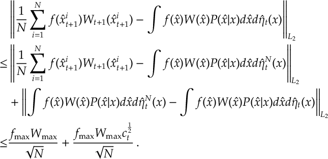
Thus for we have

$\begin{aligned} & \left\| \frac{1}{N} \sum_{i=1}^N f(\hat x_{t+1}^i) W_{t+1}(\hat x_{t+1}^i) - \int f(\hat x) W(\hat x)P(\hat x| x) d \hat x d \hat \eta_{t} (x) \right\|_{L_2} \notag \\ \leq & \left\| \frac{1}{N} \sum_{i=1}^N f(\hat x_{t+1}^i) W_{t+1}(\hat x_{t+1}^i) - \int f(\hat x) W(\hat x)P(\hat x| x) d \hat x d \hat \eta^N_{t} (x) \right\|_{L_2} \notag \\ & + \left\| \int f(\hat x) W(\hat x)P(\hat x| x) d \hat x d \hat \eta^N_{t} (x) - \int f(\hat x) W(\hat x)P(\hat x| x) d \hat x d \hat \eta_{t} (x) \right\|_{L_2} \notag \\ \leq & \frac{f_{\max}W_{\max}}{\sqrt{N}} + \frac{f_{\max} W_{\max}c^{\frac{1}{2}}_t}{\sqrt{N}}\, . \label{MC:SNI01}\end{aligned}$

The first term in follows by the same argument that we used to derive . The second term follows by our induction hypothesis applied to the function $\tilde f(x) = \int f(\hat x) W( \hat x) P(\hat x|x)d\hat x$ . Thus, applying the above inequality to (and ), we see that

$\begin{aligned} \left\| \int f(x) d \hat \eta^N_{t+1} (x) - \int f(x) d \hat \eta_{t+1} (x) \right\|_{L_2} \leq 2 \frac{f_{\max}W_{\max}}{\sqrt{N}} + 2\frac{f_{\max} W_{\max}c^{\frac{1}{2}}_t}{\sqrt{N}}\end{aligned}$

Thus we see that the require bound holds at time $t+1$ with $\begin{aligned} c_{t+1} := 4(1+c^{\frac{1}{2}}_t)^2\,.\end{aligned}$ This completes the induction step and the proof. $\square$