A Short Discussion on Policy Gradients in Bandits

This is a quick note on policy gradients in bandit problems. There are a number of excellent papers coming out on the convergence of policy gradients [1 ,2, 3]. I wrote this sketch argument a few months ago. Lockdown and homeschooling started and I found I did not have time to pursue it. Then yesterday morning I came across the following paper Mei et al. [1], which uses a different Lyapunov argument to draw an essentially the same conclusion [first for bandits then for general RL]. Although most of the time I don’t talk about my own research on this blog, I wrote this short note here just in case this different Lyapunov argument is of interest.

Further, all these results on policy gradient are [thus far] for deterministic models. I wrote a short paper that deals with a stochastic regret bound for a policy gradient algorithm much closer to projected gradient descent, again in the bandit setting. I’ll summarize this, as it might be possible to use it to derive stochastic regret bounds for policy gradients more generally. At the end, I discuss some issues around getting some proofs to work in the stochastic case and emphasize the point that $1/q^\star$ is a good choice of lyapunov function [where $latex $q^\star$ is the probability of not choosing the optimal action.]

We consider a multi-arm bandit setting. Here there are a finite set of arms $\mathcal A$ . At each time you can choose one arm $a\in\mathcal A$ and you receive a reward $R_a$ which we assume is an independent $\{0,1\}$ random variable with mean $r_a$ . You only get to see the reward of the arm that you choose and over time you want to move towards choosing the optimal [highest reward] arm.

A policy gradient algorithm is an algorithm where you directly parameterize the probability of playing each arm and then you perform a gradient descent/stochastic approximation update on these parameters. The most popular parameterization is soft-max: here the probability of playing arm $a$ is

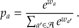
Here there are the weights $w_a$ , $a\in\mathcal A$ are applied to each arm. A quick calculation gives that

where here $I_{aa'}$ is the indicator function for $a=a'$ , i.e. $I_{aa'}=1$ if $a=a'$ and $I_{aa'}=0$ otherwise.

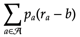
We want to maximize expected the reward (plus or minus a constant $b$ )

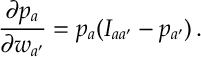
So given the last two expressions, for each arm $a$ , you can then perform the following stochastic gradient update:

where $R$ is the reward of the arm played; $B$ is some baseline [which is a function that does not depend on $a$ ]; $A$ is the index of the arm that was played; $\alpha$ is the learning rate of the algorithm.

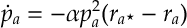
If we can model change in these weights over time with the following o.d.e.

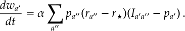
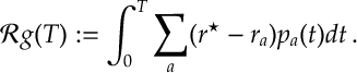
Here we let $r^\star$ be the reward of the optimal arm [Note this term does not play a role the dynamics of our model but will be useful for analyzing regret.] The regret of the algorithm is defined to be

This measures how much reward has been lost by not playing the optimal arm.

Given the above we also define

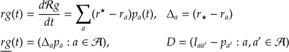
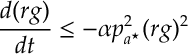
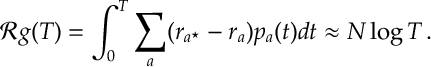
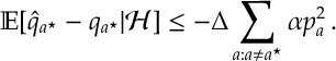
The following short argument bounds the change in the regret:

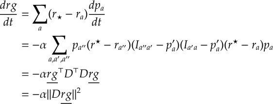
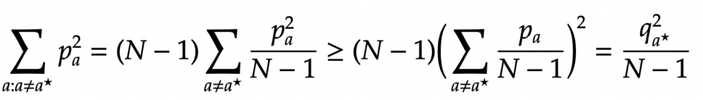
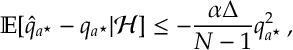
Let’s analyze the above term

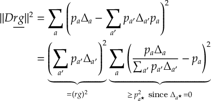
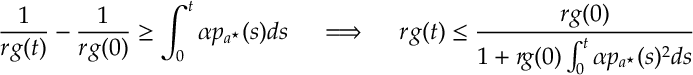
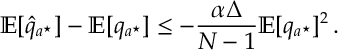
Therefore we have the bound

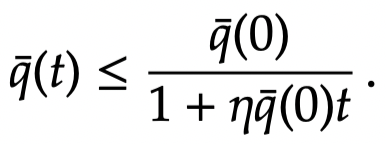
Dividing by $-(rg)^2$ and integrating gives

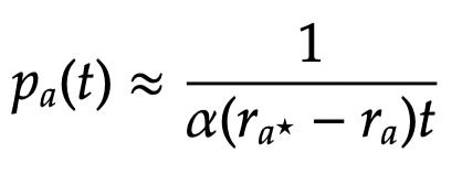
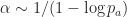
So notice things depend on the probability of playing the optimal arm. Assuming all arms start are equal the optimal arm $a^\star$ will increase from $\frac{1}{N}$ where $N$ is the number of arms. Thus we get a bound:

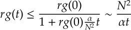
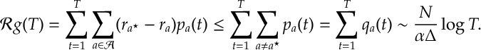
Thus we have

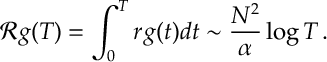
(Notice the dependence on $N$ is very pessimistic since $p_{a^\star} \rightarrow 1$ . Also note the lower-bound on $p_{a^\star}$ is more rigorously bounded in [1] and [2] below)

Stochastic Regret Bounds

So do these sorts of convergence results flesh out when we allow for stochastic effects. A proof for a slightly different policy works, and I’ll sketch out the main argument then the technical issues.

First convergence for probabilities can’t go faster than $\frac{1}{t}$ as we know the regret of bandit problems is $\log T$ . [For RL, it would seem that the similar probabilities should converge at $\frac{1}{t}$ if actions belong to the boundary and $\frac{1}{\sqrt{t}}$ if they belong to an interior stationary point. Though I don’t have a proof for this other than s.d.e. heuristics.] Notice the algorithm above optimizes the following update when parameterize $p_a$ with a soft-max objective.

We can just not reparameterize and apply projected gradient descent.

SAMBA. Analogous to the soft-max discussion above. This is how to derive a stochastic policy gradient algorithm in this case. [Projected] Gradient descent the perform the update 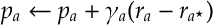for $a\neq a^\star$ . However, since the mean rewards $r_a, a\in \mathcal A,$ are not known, a stochastic gradient descent must be considered: $p_a \leftarrow p_a + \gamma (R_a-R_{a^\star})$ , $a\neq a^\star$ . Also, the optimal arm is unknown. So instead of $a^\star$ , we let $a_\star$ be the arm for which $p_a$ is maximized and, in place, consider the update $p_a \leftarrow p_a + \gamma (R_a-R_{a_\star})$ , $a\neq a_\star$ . Since the reward from only one arm can be observed at each step, we apply importance sampling:

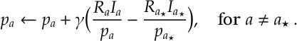
This gives a simple recursion for a multi-arm bandit problem. A name for this is SAMBA: stochastic approximation multi-arm bandit. Catchy acronyms aside, one can see this is really a stochastic gradient descent algorithm with some correction to make sure we don’t get too close to the boundary. Shortly, I’ll argue that we need to let $\gamma$ depend on $a$ and we should take $\gamma_a =\alpha p_a^2$ for $\alpha$ suitably small. A motivation is projected gradient descent or barrier methods in optimization [there is probably a regularization interpretation as well]. For policy gradients some form of projection/barrier seems to be required to maintain exploration. The general forms that work seems to be an important open problem.

Learning rate and o.d.e. analysis. Let’s consider the learning rate 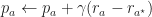$\gamma$ . Again, consider the gradient descent update $p_a \leftarrow p_a + \gamma (r_a-r_{a^\star})$ , for $a\neq a^\star$ . Notice if we let $\gamma = \alpha p_a^2$ then the gradient descent algorithm approximately obeys the following differential equation:

whose solution is

This implies

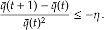
This suggest a learning rate of $\gamma = \alpha p_a^2$ , applied to each $a$ , gives a logarithmic regret.

Discrete time analysis. A discrete time version of the above result is the following lemma

Lemma. If $(\bar q(t) : t\in\mathbb Z_+)$ is positive with

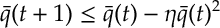
for some $\eta >0$ , then

A proof of this is given at the end of this post.

martingale analysis. Notice if we let $\hat p_a$ be the update on the right-hand side of then the expected change in the update [given history $\mathcal H$ ] is

If we define $q_{a^\star} = 1-p_{a^\star}$ , summing over $a\neq a^\star$ gives

where $\Delta = \min_{a\neq a^\star} \Delta_a$ .

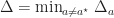
By Jensen’s inequality:

Thus applying the above bound gives

Here we have a positive super-martingale, so by Doob’s Martingale Convergence Theorem $q_{a^\star}$ converges as time goes to infinity. With a few standard tricks you can show the limit must be zero. We can get a rate of convergence from the discrete time analysis above. Taking expectations and applying Jensen’s inequality one more time gives:

Thus the lemma above gives

which then leads the following stochastic regret bound

Discussion on Convergence Issues. Both soft-max and SAMBA step rules require some form of best arm identification. For SAMBA this is explicit in that we need $a_{\star}$ the highest probability arm to equal the optimal arm $a^\star$ . [And a lot of the technical leg work in our paper involves proving this happens]. For soft-max it is clear that if $p_{a^\star}$ gets small for a sustained period of time then this slows convergence. So in both cases we need $p_{a^\star}$ to get big in a reasonable length of time. This argument is more straight-forward in the o.d.e case where we can bound $p_{a^\star}$ away from zero by a constant. In the stochastic case we need sub-martingale arguments to do this for us. And this can be fiddly as we are essentially dealing with a random walk that is close to threshold between recurrence and transience.

One thing that seems to come out of the analysis for both soft-max [when you include 2nd order terms] and SAMBA is that if the learning rate is too big then then this random walk switches from being transient [and thus converging on the correct arm] to being recurrent [and thus walking around the interior of the probability simplex within some region of the optimal arm]. One way to deal with this is to slow decrease the learning rate either as a function of either time $\alpha \sim 1/\log t$ or as a function of the state $\alpha \sim 1/(1-\log p_a)$ . This appears to multiply on an extra $\log t$ term on the regret bound in both cases while guaranteeing global convergence in the bandit setting. We can consider more slowly decreasing functions which impact regret to an arbitrarily small amount. So it seems like there is a regret of $(\log T)^{1+\epsilon}$ for $\epsilon$ arbitrarily small.

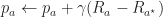
A final point is that in all the analysis so far [both softmax and SAMBA], we have used an o.d.e. of the form

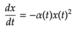
which suggests that we apply a Lyapunov function of the form:

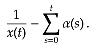
Proving martingales properties for these Lyapunov functions seems to be a key ingredient for getting stochastic proofs to work.

Appendix.

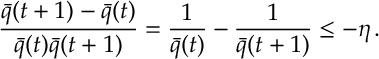
Proof of Lemma. Dividing the expression by $\bar q(t)^2$ gives

Since $\bar q(t+1)$ is less than $\bar q(t)$ but still positive, dividing by $\bar q(t+1)$ rather that $\bar q(t)$ decreases the previous lower bound

Summing from $t=1,...,T-1$ gives

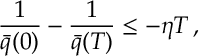
which rearranges to give

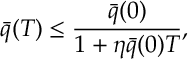
as required.

References

Mei J, Xiao C, Szepesvari C, Schuurmans D. On the Global Convergence Rates of Softmax Policy Gradient Methods. arXiv preprint arXiv:2005.06392. 2020 May 13.
Agarwal, A., Kakade, S. M., Lee, J. D., and Mahajan, G. Optimality and approximation with policy gradient methods in markov decision processes. arXiv preprint arXiv:1908.00261, 2019.
Bhandari J, Russo D. Global optimality guarantees for policy gradient methods. arXiv preprint arXiv:1906.01786. 2019 Jun 5.

Stochastic Regret Bounds

Appendix.

References

Share this:

Like this:

Leave a Reply Cancel reply