Algorithms for MDPs

High level idea: Policy Improvement and Policy Evaluation.
Value Iteration; Policy Iteration.
Temporal Differences; Q-factors.

For infinite time MDPs, we cannot apply to induction on Bellman’s equation from some initial state – like we could for finite time MDP. So we need some algorithms to solve MDPs.

At a high level, for a Markov Decision Processes (where the transitions $P^{a}_{xy}$ are known), an algorithm solving a Markov Decision Process involves two steps:

(Policy Improvement) Here you take your initial policy $\pi_0$ and find a new improved new policy $\pi$ , for instance by solving Bellman’s equation:

$\pi(x) \in \argmax_{a\in \mathcal A} \left\{ r(x,a) + \beta \mathbb{E}_{x,a} \left[ R(\hat{X},\pi_0) \right] \right\}$

(Policy Evaluation) Here you find the value of your policy. For instance by finding the reward function for policy $\pi$ :

$R(x,\pi) = \mathbb E^\pi_{x} \left[ \sum_{t=0}^\infty \beta r(X_t,\pi(X_t))\right]$

Value iteration

Value iteration provides an important practical scheme for approximating the solution of an infinite time horizon Markov decision process.

Def. [Value iteration] Take $V_0(x)=0$ $\forall x$ and recursively calculate

$\begin{aligned} \pi_{s+1}(x) \in & \argmax_{a\in {\mathcal A} } \left\{ r(x,a) + \beta \mathbb{E}_{x,a} \left[ V_s(\hat{X}) \right] \right\} \\ V_{s+1}(x) & = \max_{a\in {\mathcal A} } \left\{ r(x,a) + \beta \mathbb{E}_{x,a} \left[ V_s(\hat{X}) \right] \right\}\end{aligned}$

for $s=1,2,..$ this is called value iteration.

We can think of the two display equations above, respectively, as the policy improvement and policy evaluation steps. Notice, that we don’t really need to do the policy improvement step to do each iteration. Notice the policy evaluation step evalutes one action under the new policy $\pi$ afterwards the value is $V_s(\hat{X})$ .

Similarly we can define value iteration for minimization problem:

$L_{s+1}(x) = \min_{a\in {\mathcal A} } \left\{ l(x,a) + \beta \mathbb{E}_{x,a} \left[ L_s(\hat{X}) \right] \right\}.$

Each iteration of value iteration improves the solution:

Ex 1. For reward function $R(x)$ define

$\mathcal L R(x) = \max_{a\in {\mathcal A} } \left\{ r(x,a) + \beta \mathbb{E}_{x,a} \left[ R(\hat{X}) \right] \right\}.$

Show that if $R(x) \geq \tilde{R}(x)$ for all $x\in \mathcal X$ then $\mathcal L R(x) \geq \mathcal L \tilde{R}(x)$ for all $x\in \mathcal X$ .

Ans 1.

$r(x,a) + \beta \mathbb{E}_{x,a} \left[ R(\hat{X}) \right] \geq r(x,a) + \beta \mathbb{E}_{x,a} \left[ \tilde{R}(\hat{X}) \right].$

Now maximize both sides over $a\in\mathcal A$ .

Ex 2. [Continued] Show that for value iteration with positive programming

$V_{s+1}(x) \geq V_s(x)$

Ans 2. $V_1(x) = \max_a r(x,a) \geq 0 = V_0(x).$ Now repeatedly apply [1].

Ex 3. [Continued][IDP:Cont_2] Show that for value iteration with negative programming

$L_{s+1}(x) \leq L_s(x).$

Ans 3. Identical idea as [1-2].

So we know Value Iteration improves the value function on each step. We now need to argue the value iteration gets to the optimal solution.

Ex 4. Show that for discounted programming

$\lim_{s\rightarrow \infty} V_s(x) = V(x)$

Ans 4. Note that $V_{s+1}$ is the optimal solution to the finite time MDP with $s+1$ steps, recall in Def [MDP:Def]. Thus,

$V_{s}(x) + \frac{\beta^{s+1} r_{\max} }{1-\beta} \geq V(x) \geq V_{s}(x)$

Now let $s\rightarrow\infty$ .

Ex 5. Show that for positive programming

$\lim_{s\rightarrow \infty} V_s(x) = V(x)$

Ans 5. Take any policy $\Pi$ . Then

$V_s(x) \geq R_s(x,\Pi)$

Now take limits $V_{\infty}(x) \geq R(x,\Pi)$ . Now maximize over $\Pi$ .

Ex 6. Show that for negative programming with a finite number of actions

$\lim_{s\rightarrow \infty} L_s(x) = L(x)$

Ans 6. Same idea as [5].

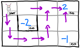
Ex 7. [GridWorld] A robot is placed on the following grid.

The robot can chose the action to move left, right, up or down provided it does not hit a wall, in this case it stays in the same position. (Walls are colored black.) With probability 0.8, the robot does not follow its chosen action and instead makes a random action. The rewards for the different end states are colored above. Write a program that uses, Value Iteration to find the optimal policy for the robot. Grid

Ans 7. Notice that the robot does not just take the shortest root. (I.e. some forward planning is required)

Policy Iteration

We consider a discounted program with rewards $r(x,a)$ and discount factor $\beta \in (0,1)$ .

Def 2. [Policy Iteration] Given the stationary policy $\Pi$ , we may define a new (improved) stationary policy, ${\mathcal I}\Pi$ , by choosing for each $x$ the action ${\mathcal I}\Pi (x)$ that solves the following maximization

${\mathcal I}\Pi (x) \in \argmax_{a\in{\mathcal A} } \; r(x,a) + \beta \mathbb{E}_{x,a} \left[ R(\hat{X},\Pi) \right]$

where $R(x,\Pi)$ is the value function for policy $\Pi$ . We then calculate $R(x,\mathcal I \Pi)$ . Recall that for each $x$ this solves the equations

$R(x,\mathcal I \Pi) = r(x,\mathcal I \Pi (x)) + \beta \mathbb{E}_{x,a} \left[ R(\hat{X},\mathcal I \Pi) \right]$

Policy iteration is the algorithm that takes

$\Pi_{n+1} = {\mathcal I} \Pi_n$

Starting from some of the tree stationary policy $\Pi_0$ .

Thrm 1. Under Policy Iteration

$R(x,\Pi_{n+1}) \geq R(x,\Pi_n)$

and, for bounded programming,

$R(x,\Pi_n) \nearrow V(x) \qquad \text{as} \quad n \rightarrow \infty$

Ex 8 [Proof of Thrm 1] Under the policy iteration

$R(x,{\mathcal I}\Pi ) \geq R(x,\Pi)$

(Hint: requires Ex 8 & Ex 10 from Markov Chains)

Ans 8. By Ex 8 from Markov Chains, and the optimality of $\mathcal I \Pi$ with respect to $\Pi$ we have

$\begin{aligned} R(x,\Pi) = r(x,\pi(x)) + \beta \mathbb E_{x,\pi(x)} \left[ R(\hat{X},\Pi) \right] \leq r(x,\mathcal I \Pi (x)) + \beta \mathbb E_{x,\mathcal I \pi(x)} \left[ R(\hat{X},\Pi) \right]\end{aligned}$

Applying Ex 10 from Markov Chains gives the result.

Ex 9. [Continued]

$r(x,a) + \beta \mathbb E_{x,a} \left[ R(\hat{X},\Pi) \right] \geq R(x,\mathcal I \Pi)$

Ans 9.

$\begin{aligned} r(x,a) + \beta \mathbb E_{x,a} \left[ R(\hat{X},\Pi) \right] & \leq r(x,\mathcal I \pi(x)) + \beta \mathbb E_{x,\mathcal I(x)} \left[ R(\hat{X},\Pi) \right] \\ & \leq r(x, \mathcal I \pi(x)) + \beta \mathbb E_{x,\mathcal I \Pi} \left[ R(\hat{X},\Pi) \right] = R(x,\mathcal I \Pi) \end{aligned}$

We now proceed via a Martingale argument. Define $M_t = \beta^t R(X_t,\Pi_{T-t}) + \sum_{s=0}^{t-1} \beta^s r(X_s,\pi^*(X_s))$

where $\pi^*(x)$ is the optimal policy.¹

Ex 10. [Continued] Show that $M_t$ is a supermartingale with respect to $\Pi^*$ .

Ans 10. Taking expectations with respect to the optimal policy $\Pi^*$

$\begin{aligned} &\mathbb E^* \left[ M_{t+1} - M_t | \mathcal F_t \right] \\ & = \beta \mathbb E^* \left[ \beta R(X_{t+1},\Pi_{T-t-1}) + r(X_t, \pi^*(X)t) - R(X_t,\Pi_{T-t}) \Big| \mathcal F_t \right] \\ & = \beta^t \mathbb E^* \left[T \beta \mathbb E^*_{X_t,\pi^*(X_t)} \left[ \beta R(\hat{X},\Pi_{T-t-1}) + r(X_t,\pi^*(X_t)) - R(X_t,\Pi_{T-t}) \right] \Big| \mathcal F_t \right] \\ & \geq 0\end{aligned}$

The inequality at the end follows by [9].

Ex 11. [Continued]

$R(x,\Pi_n) \nearrow V(x)\qquad \text{as} \quad n\rightarrow \infty.$

Ans 11. Since $M_t$ is a supermartingale:

$\begin{aligned} R(x,\Pi_T) = \mathbb E^*_x \left[ M_0 \right] \geq \mathbb E^*_x \left[ M_T \right] = \underbrace{ \mathbb E^*_x \left[ \beta^T R(X_T,\Pi_0) \right] }_{ \xrightarrow[T\rightarrow \infty]{} 0 } + \underbrace{ R_T(x,\Pi^*) }_{ \xrightarrow[T\rightarrow \infty]{} V(x) }\end{aligned}$ Therefore, as required,

$\lim_{T\rightarrow \infty} R(x,\Pi_T) \geq V(x).$

Ex 12. [GridWorld, again] Write a program that uses, Policy iteration to find the optimal policy for the robot in [7].

Ans 12.

Temporal Difference Iteration

We now discuss how temporal differences, defined below, relate to value iteration and policy iteration. From define a parameterized set of policies that have value iteration and policy improvement as special cases.

Def 3 [Temporal Differences] For a MDP, reward function $R$ , and an action $a$ , the temporal differences are

$d_{a}(x,y) = r(x,y, a) + \beta R(y) - R(x)$

The following exercises show that the Bellman equation and the definition of a stationary policy can be phrased in terms of temporal differences.

Ex 13. [Bellman Equation with Temporal Differences] Show that if $R$ is not optimal value function then

$\max_{a\in \mathcal A}\left\{ \mathbb E_{x,a} \left[ d_a(x,\hat{X}) \right] \right\} \geq 0.$

Ex 14. [Continued] Show that if $R$ is optimal value function then

$\max_{a\in \mathcal A}\left\{ \mathbb E_{x,a} \left[ d_a(x,\hat{X}) \right] \right\} = 0.$

Ex 15. [Stationary rewards] Show that the reward function for a stationary policy $\pi$ satisfies,

$\mathbb E_{x,\pi} \left[ d_{\pi(x)}(X_0,{X}_1) \right] =0,\qquad x\in \mathcal X.$

We now consider how temporal differences are used to update our value function in value iteration and policy iteration.

Ex 16. [Policy improvement] Show that policy improvement for value iteration and policy iteration are given by

$\pi(x) = \argmax_{a\in \mathcal A} \mathbb E_{x,a} \left[ d_a(x,\hat{X})\right]$

Ex 17. [Continued, Value iteration] Show that policy evaluation under value iteration, updates the value function $R=V_0$ to $V$ according to

$V(x) = V_0(x) + \mathbb E_{x,\pi(x)} \left[ d_a(x,\hat{X})\right]$

where $\pi(x)$ is as given in the policy improvement step.

(i.e. the temporal difference gives the change in the value function.)

Ex 18. [Continued, Policy Iteration] Show that policy evaluation under policy improvement, update that value function $R=V_0$ to $V$ according to

$V(x) = V_0(x) + \mathbb E_{x,\pi} \left[ \sum_{t=0}^\infty \beta^t d(X_t,X_{t+1}) \right]$

Lambda-Policy Improvement

Notice that both value iteration and policy improvement have exactly the same policy improvement step:

${\pi} (x) \in \argmax \Big\{ r(x,a) + \beta \mathbb E_{x,a} \left[ V_0(x)\right]\Big\}$

where $V_0(x)$ is the value attributed to the previous policy. However, they differ in how the evaluate the policy. In particular, value iteration considers one step under the new policy:

${V}(x) := \mathbb E^{{\pi}}_{x} \left[ r(X_0,{\pi}(X_0)) + \beta V_0({X}_1) \right],$

where as policy iteration takes an infinite number of steps:

${V}(x) := \mathbb E^{\pi} \left[ r(X_0,{\pi}(X_0)) + \beta r(X_1,{\pi}(X_1)) + \beta^2 r(X_2,{\pi}(X_2)) +\dots \right].$

The Temporal Difference method takes a geometrically distributed² number of steps:

$V(x) := \mathbb E^{\pi} \left[ \sum_{t=0}^{\tau_\lambda} \beta^t r(X_t,\pi(X_t)) + \beta^{\tau_\lambda + 1} V_0(X_{\tau_\lambda + 1}) \right].$

where $\tau_\lambda$ is a geometrically distributed random variable on $\mathbb Z_+$ with probability of success $(1-\lambda$ ).

Ex 19. [Value function from switching policies] Let $V^{(0)}(x)$ be value function of a stationary policy $\Pi^{(0)}$ and let $V^{(1)}(x)$ be value function of a stationary policy $\Pi^{(1)}$ .

Let $\Pi^{(\lambda)}$ be the policy that follows $\Pi^{(1)}$ for a geometrically distributed time with success probability $1-\lambda$ and there after follows policy $\Pi^{(0)}$ . Show that the value function of $\Pi^{(\lambda)}$ satisfies

$V^{(\lambda)} (x) = \mathbb E^{\pi} \left[ \sum_{t=0}^{\tau_\lambda-1} \beta^t r(X^{(1)}_t,\pi^{(1)}(X^{(1)}_t)) + \beta^{\tau_\lambda } V_0\big(X^{(1)}_{\tau_\lambda }\big) \right].$

Ans 19. Should be obvious from discussion above.

Ex 20. [Continued, Bellman Equation] Argue that $V^{(\lambda)}$ also satisfies the recursion

$V^{(\lambda)} (x) = r(x,\pi^{(1)}(x)) + \beta \mathbb E_{x,\pi^{(1)}(x)} \left[ \lambda V^{(\lambda)}(\hat{X}) + (1-\lambda) V^{(0)} (\hat{X}) \right]$

Ans 20. [ADP:TD_1] This is recursion for the value function of this Markov chain, see [8] from Markov Chains. At each jump, with probability $\lambda$ , $X^{(1)}$ continues and, with probability $1-\lambda$ , $X^{(1)}$ stops and takes value $V^{(0)}(\cdot)$ .

Ex 21. [Continued, relation with Temporal Differences] Show that $V^{(\lambda)} ( x) = V^{(0)} (x) + \sum_{t=0}^\infty \beta^t \lambda^t \mathbb E\left[ d_{\pi^{(0)}} ( X_t, X_{t+1} ) \right]$

Ans 21. We use the shorthand $r_t=r(X^{(1)}_t,\pi^{(1)}(X^{(1)}_t))$ & $V_t^{(0)}=V^{(0)}(X^{(0)}_t)$ . From [19],

$\begin{aligned} V^{(\lambda)}(x) & = \mathbb E \left[ \sum_{t=0}^\infty \mathbb I [ \tau_\lambda > t ] \beta^t r_t + \sum_{t=0}^\infty \mathbb I [\tau_\lambda = t ] \beta^t V^{(0)}_t \right] \\ & = \sum_{t=0}^\infty \lambda^t \beta^t\mathbb E [r_t] + \sum_{t=1}^\infty (1-\lambda)\lambda^{t-1} \beta^t V^{(0) }_t \\ & = \sum_{t=0}^\infty \lambda^t \beta^t\mathbb E [r_t] + \beta \sum_{t=0}^\infty \lambda^t \beta^t V^{(0)}_{t+1} - \sum_{t=1}^\infty \lambda^t \beta^t V^{(0)} \\ & = V^{(0)}(x) + \sum_{t=0}^\infty \lambda^t \beta^t \mathbb E \left[ d(X_t,X_{t+1})\right].\end{aligned}$

Q-factors

Def 4. [Q-Factor] The $Q$ -factor of a stationary policy $\pi$ is the from taking action $a$ and then following policy $\pi$ there after, that is

$Q_\pi(x,a) = \mathbb E_{x,a} [ r(x,a) + \beta R(\hat{X},\pi))]$

The Q-factor (of the optimal policy) is given by

$Q^*(x,a) =\max_{\pi} Q_{\pi}(x,a).$

Ex 22. Show that stationary $Q$ -factors satisfy the recursion $Q_\pi(x,a) = \mathbb E_{x,a} [ r(x,a) + \beta Q_{\pi}(\hat{X},\pi(\hat{X}) )]$

Ex 23. Show that Bellman’s Equation can be re-expressed in terms of $Q$ -factors as follows

$Q^*(x,a) = \mathbb E_{x,a} [ r(x,a) + \beta \max_{\hat{a}} Q^*(\hat{X},\hat{a}) )]$

Ex 24. Show that the optimal value function satisfies

$V(x) = \max_{a\in \mA} Q^*(x,a).$

Note we are implicity assuming an optimal stationary policy exists. We can remove this assumption by considering a $\epsilon$ -optimal (non-stationary) policy. However, the proof is a little cleaner under our assumption.↩
By keeping things geometrically distributed we preserve the Markov property. This would not hold for other distributions↩