A short introduction to Markov chains for dynamic programming
Definition, Markov Property, some Potential Theory.

Markov Chains

Introductory example: snakes and ladders

We highlight some of the key properties of Markov chains: how to calculate transitions, how the past effects the current movement of the processes, how to construct a chain, what the long run behavior of the process may (or may not) look like. We give an initial example to better position our intuition.

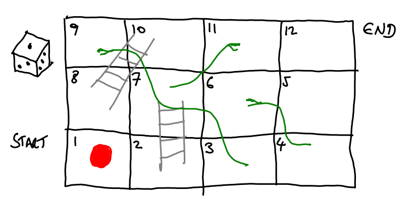
Below in Figure [Snakes_and_ladders], we are given a game of snakes and ladders (or shoots and ladders in the US). Here a counter (coloured red) is placed on the board at the start. You roll a dice. You move along the numbered squares by an amount given by the dice. The objective is to get to the finish. If the counter lands on a square with a snake’s head, you must go back to the square at the snakes tail and, if you land on a square at the bottom of a ladder, go to the top of the ladder.

[Snakes_and_ladders]

We let $X_t$ be the position of the counter on the board after the dice has been thrown $t$ times. The processes $X=(X_t: t\in {\mathbb Z})$ is a discrete time Markov chain. The following exercises should be fairly straight-forward.

Ex 1 [Transition Probabilities] Given that the counter is in square $x$ we let $P_{xy}$ be the probability that you next go to square $y$ . I.e.

$P_{xy}={\mathbb P}(X_1=y | X_0 =x).$

Calculate:

a) $P_{14}$ b) $P_{17}$ c) $P_{34}$

Ans 1 a) $1/3$ b) $1/3$ c) $1/3$ .

Ex 2 [Continued] Calculate

a) ${\mathbb P}(X_1=7|X_0=6)$ b) ${\mathbb P}(X_3=7|X_2=6)$

c) ${\mathbb P}(X_2 = 5, X_1=3 | X_0=1)$ d) ${\mathbb P}(X_2=5| X_1=1)$ .

Express your answer both numerically and in terms of sum of multiples of $P_{xy}$ .

(Note that many probabilities can be calculated via matrix multiplication on $P$ .)

Ans 2

a) $P_{67}=1/3$

b) $P_{67}=1/3$

(Nb. the fact the process started at time $2$ does not effect the probability).

c) $P_{13}P_{35}=1/6 \cdot 1/6 = 1/36$

(Nb. For times and states in series we just multiply entries)

d) $\sum_j P_{1j}P_{j5} = P_{13}P_{35}+P_{14}P_{45} = 1/18$ . (Nb. We have to sum over entries for times that we miss out) (Nb. Also, note that $\sum_j P_{1j}P_{j5}$ is the $(1,5)$ entry of the matrix $P^2$ ).

Ex 3 [Markov property] Show that

$\begin{aligned} {\mathbb P} (X_3=7 | X_2=6, X_1=3,X_0=1 ) = & {\mathbb P} (X_3=7 | X_2=6, X_1=5,X_0=1 ) \\ = & {\mathbb P} (X_3=7 | X_2=6 )\end{aligned}$

We see that given we are on square $6$ , the probability of reaching square $7$ is not effected by the path by which we reached square $6$ .

Ans 3

$\begin{aligned} \mathbb P (X_3=7 | X_2=6, X_1=3,X_0=3 ) & = \frac{ \mathbb P (X_3=7, X_2=6, X_1=3 | X_0=1 ) }{ \mathbb P ( X_2=6, X_1=3 | X_0=1 ) } \\ & = \frac{1/6 \cdot 1/6 \cdot 1/3}{1/6 \cdot 1/3} \end{aligned}$

The calculation for ${\mathbb P} (X_3=7 | X_2=6, X_1=5,X_0=1 )$ is very similar and ${\mathbb P} (X_3=7 | X_2=6 )$ is [[MC:Ladders2]] part b).

In general, given that counter is on a square we will see that the next square reached by the counter on the next turn is not effected by the path that was used to reach the square. This is called the Markov Property.

Ex 4 [Jump chain construction] Convince yourself that if you were given the current square of the Markov chain $X_0=x$ and the throw of the dice $U_1=u$ , then this completely determines the next square $X_{1}=y$ .

This give a method for constructing and simulating Markov chains. We just need to keep track of the current state and generate an independent random variable to determine the next state.

Ans 4 Note that this essentially says that

$X_{t+1}= F(X_t ; U_t)$

for some function $F(x;u)$ .

Certainly there is more than one could say here. However we will cover more in future exercises with a formal definition in place.

Markov Chain Definition

Let $\mathcal{X}$ be a countable set.

Def [Initial Distribution/Transition Matrix] An initial distribution

$\lambda=(\lambda_x: x\in\mathcal{X})$

is a positive vector whose components sums to one. A transition matrix $P=(P_{xy} : x,y\in\mathcal{X})$ is a postive matrix whose rows sum to one, that is, for $x\in\mathcal{X}$

$\sum_{y\in\mathcal{X}} P_{xy}=1.$

Def [Discrete Time Markov Chain] We say that a sequence of random variables $X=(X_t:t\in\mathbb{Z}_+)$ is a discrete time Markov chain, with initial distribution $\lambda$ and transition matrix $P$ if for $x_0,...,x_{t+1}\in\mathcal{X}$ ,

$\begin{aligned} \mathbb{P}(X_0=x_0)=\lambda_0\end{aligned}$

and

ba12b6ec66c2e702da0bb6de7fa22048

The first equality above is often called the Markov property and is the key defining feature of a Markov chain or, more generally, Markov process. It states that the past $(X_1,...,X_{t-1})$ and future $X_{t+1}$ are conditionally independent of the present $X_t$ . Otherwise stated, is says that, when we know the past and present states $(X_1,...,X_t)=(x_0,...,x_t)$ , the distribution of the future states $X_{t+1}, X_{t+2},...$ is only determined by the present state $X_t=x_t$ . Think of a board game like snakes and ladders, where you go in the future is only determined by where you are now and not how you got there; this is the Markov property.

Ex 5 [Constructing Markov Chains] Take a function $f:\mathcal{X}\times [0,1] \rightarrow \mathcal{X}$ , $X_0$ a random variable on $\mathcal{X}$ , and $(U_t)_{t\geq 0}$ , independent uniform $[0,1]$ random variables. Construct the sequence $(X_t)_{t\geq 0}$ with the recursion

$X_{t+1}=f(X_t,U_t) \qquad\text{ for} \quad t=0,1,2,..$

Show $(X_t)_{t\geq 0}$ that is a discrete time Markov chain.

Ex 6 [continued] Show that all discrete time Markov chains can be constructed in this way.

Ex 7 [Markov Chains and Martingale Problems] Show that a sequence of random variables $X=(X_t : t\in\mathbb{Z}_+)$ is a Markov chain if and only if, for all bounded functions $f:\mathcal{X} \rightarrow \mathbb{R}$ , the process

$M^f_t = f(X_t) - f(X_0) - \sum_{\tau =0}^{t-1} (P-I)f(X_\tau)$

is a Martingale with respect to the natural filtration of $X$ . Here for any matrix, say $Q$ , we define

$Qf(x) := \sum_{y\in\mathcal{X}} Q_{xy} f(y) .$

Markov Chains & Potential Theory

This is really just more resolvants.

Ex 8 [Markov Chains and Potential Functions] Let $r:\mathcal{X}\rightarrow \mathbb{R}_+$ be a bounded function. Argue that for $\beta \in (0,1)$

$R(x) = \mathbb{E}_x \left[ \sum_{t=0}^{\infty} \beta^t r(X_t) \right]$

solves the equation

$%\label{MC:Resolve} R(x) = \beta (PR) (x) + r(x), \qquad x\in\mathcal{X}.$

Ans 8

$R(x) = r(x) + \mathbb{E}_x \bigg[ \beta \mathbb{E}\bigg[ \sum_{t=1}^\infty \beta^{t-1} r(X_t)\Big| X_1\bigg]\bigg]=r(x) + \mathbb{E}_x\bigg[\beta R(X_1)\bigg] = r(x)+\beta (PR)(x)$

Ex 9 [Continued][MC:Potential1.2] Show that $R$ is the unique bounded solution this equation.

Ans 9 Take any $\hat{R}$ then $\hat{R}-R=\beta P(\hat{R}-R)$ . So

$|| \hat{R}-R ||_\infty \leq \beta \sum_y P_{xy} |R(y) - R(y) | \leq \beta || \hat{R} -R||_\infty$

which, since $\beta <1$ , only holds if $\hat{R} = R$ .

Ex 10 [Continued] Show that if the bounded function $\tilde{R}:\mathcal{X} \rightarrow \mathbb{R}_+$ satisfies

$\tilde{R}(x) \geq \beta (P\tilde{R}) (x) + r(x), \qquad x\in\mathcal{X}.$

then $\tilde{R}(x) \geq R(x)$ , $x\in\mathcal{X}$ .

Ans 10 Suppose that $\tilde{R}$ is a positive fn such that $\tilde{R}(x) \geq r(x) +\beta P\tilde{R} (x)$ . Repeated substitution gives

$\begin{aligned} \tilde{R}(x) \geq r(x) + \mathbb{E}_x\left[ \beta \tilde{R}(X_1)\right]\geq ... &\geq \mathbb{E}_x \bigg[ \sum_{t=0}^T \beta^t r(X_t) \bigg]+ \beta^{T+1} \mathbb{E}_x \bigg[\tilde{R}(X_{T+1})\bigg]\\ &\geq \mathbb{E}_x \bigg[ \sum_{t=0}^T \beta^t r(X_t)\bigg] \xrightarrow[T\rightarrow\infty]{ }R(x). \end{aligned}$

Ex 11 Let $\partial \mathcal{X}$ be a subset of $\mathcal{X}$ and let $T$ be the hitting time on $\partial\mathcal{X}$ i.e. $T=\inf\{ t : X_t \in \partial \mathcal{X}\}$ and take $f: \partial X \rightarrow \mathbb{R}_+$ argue that