Zero-Order Stochastic Optimization: Keifer-Wolfowitz

We want to optimize the expected value of some random function. This is the problem we solved with Stochastic Gradient Descent. However, we assume that we no longer have access to unbiased estimate of the gradient. We only can obtain estimates of the function itself. In this case we can apply the Kiefer-Wolfowitz procedure.

The idea here is to replace the random gradient estimate used in stochastic gradient descent with a finite difference. If the increments used for these finite differences are sufficiently small, then over time convergence can be achieved. The approximation error for the finite difference has some impact on the rate of convergence.

The Problem Setting

Suppose that we have some function $F : \mathbb R^p \rightarrow \mathbb R$

$F(\theta) = \mathbb E_U [ f (\theta ; U) ],$

that we wish to minimize over $\theta \in \mathbb R^p$ . Here $U$ is some random variable.

We suppose that we do not have direct access to the distribution of $U$ nor $f(\theta;U)$ . But we can sample $U_1,U_2,\dots$ and thus we can sample $f(\theta_1;U_1),f(\theta_2;U_2),...$ for different values of $\theta_t$ .

We can think of $f(\theta, U)$ as representing the random reward from a simulator configured under a set of parameters $\theta$ . We want to maximize the expect reward from the simulator but can only use the information of rewards from different simulation runs.

The Kiefer-Wolfowitz Algorithm

If the problem is reasonably smooth then we can use the Keifer-Wolfowitz proceedure to optimize $F(\theta)$ . Here we use a finite difference approximation of the gradient of $G(\theta)$ .

A finite difference approximation. We want to approximate the gradient of $F(\theta)$ , which we denote by $G(\theta)$ . That is

$G(\theta) := \nabla F(\theta) \, .$

We define for $\gamma \in \mathbb R$

$F(\theta + \gamma) := (F( \theta + \gamma \bm e_i ) : i =1,...,p)$

where $e_i$ is the $i$ th unit vector. We can then define the finite difference approximation to the gradient $G(\theta)$ by

$G_\gamma(\bm \theta) := \frac{F(\bm \theta + \bm \gamma ) - F(\bm \theta - \bm \gamma ) }{2\gamma}$

It is not hard to show that for a well-behaved function $F$ we have that

$G(\bm\theta) + G_{\gamma}(\bm\theta) = O( \gamma^2) \, .$

(Also note that higher-order bounds can also be used here for an improved rate of convergence.)

The Algorithm

The Kiefer-Wolfowitz Algorithm performs the update

$\label{KW:Alg} \bm\theta_{t+1} = \bm\theta_t - \bm\alpha_t \left[ \frac{f(\bm\theta_t+\bm\gamma_t,U_t)-f(\bm\theta_t-\bm\gamma_t,U_t)}{2\gamma_t} \right]$

I.e. we replace the finite difference estimate of $F( \theta)$ with the analogous random finite difference in $f( \theta,U )$ .

We need to choose $\alpha_t$ and $\gamma_t$ so that we converge to the optimum.

Assumptions

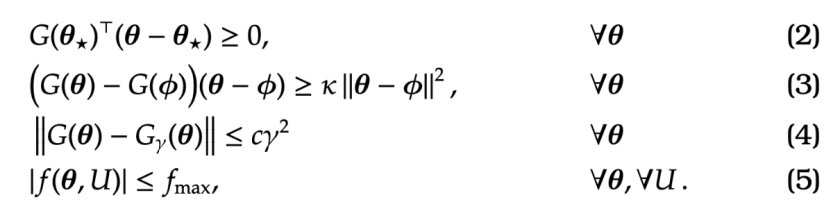
We make the following assumptions on 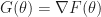$G(\theta) = \nabla F(\theta)\,$ . There exists $\theta_\star$ and there exists a constant $c$ and $f_{\max}$ such that $\begin{aligned} &G(\bm\theta_\star)^\top ( \bm\theta- \bm\theta_\star) \geq 0 , && \forall \bm\theta \label{KW:As1} \\ & \big( G(\bm\theta) - G(\bm\phi) \big)(\bm\theta -\bm\phi) \geq \kappa \left\| \bm\theta-\bm\phi \right\|^2 , && \forall \bm\theta \, \label{KW:As2} \\ & \left\| G(\bm\theta) - G_{\gamma} (\bm\theta) \right\| \leq c\gamma^2 && \forall \bm\theta \label{KW:As3} \\ & |f(\bm\theta, U)| \leq f_{\max} , && \forall \bm \theta, \forall U\, .\end{aligned}$ Notice that if $F(\theta)$ is strongly convex with its optimum at $\theta_\star$ then the two statements above follow.

Screenshot 2022-10-28 at 10.43.28

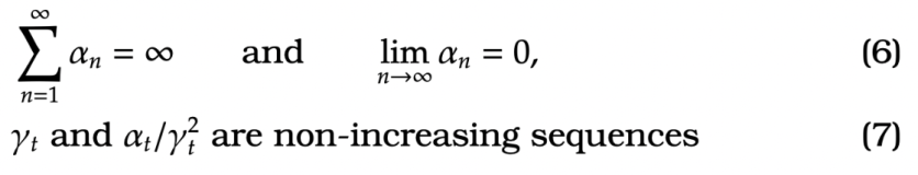
We also place assumptions on the sequences $\alpha_n$ and $\gamma_n$ specifically we assume that

Screenshot 2022-10-28 at 10.44.28 $\begin{aligned} &\sum_{n=1}^\infty \alpha_n = \infty \qquad\text{and}\qquad \lim_{n \rightarrow \infty} \alpha_n = 0, \label{KW:As4} \\ &\text{$\gamma_t$ and $\alpha_t/\gamma^2_t$ are non-increasing sequences}\label{KW:As5}\end{aligned}$

Main Result

THEOREM. For the Kiefer-Wolfowitz procedure , if (2-7) hold then

$\label{KW:thrm:eq1} \limsup_{t\rightarrow\infty} \frac{\mathbb E \left[\left\| \bm\theta_t -\bm\theta_\star \right\|^2 \right]}{\gamma_t^4 + \alpha_t / \gamma_t^2} <\infty$

Specifically if we take $\alpha_t = 1/t$ and $\gamma_t = t^{-1/6}$ then

Screenshot 2022-10-28 at 10.46.26 $\begin{aligned} \label{KW:thrm:eq2} \limsup_{t\rightarrow\infty} \frac{\mathbb E \left[\left\| \bm\theta_t -\bm\theta_\star \right\|^2\right] }{t^{2/3}} \leq \frac{1}{2} \left[ \frac{c^2}{\kappa^2} +\frac{f_{\max}^2}{4} \right] %\end{aligned}$ The proof of Theorem relies on the following proposition.

PROPOSITION. Given $\xi_n$ is a positive sequence, $b_n$ and $e_n$ are positive non-increasing sequences and $a_n$ are such that $\begin{aligned} \sum_{n=1}^\infty \alpha_n = \infty \qquad\text{and}\qquad \lim_{n \rightarrow \infty} \alpha_n = 0, %\end{aligned}$ if

$\xi_{n+1} \leq \xi_n (1 -a_n) + a_n b_n \xi^{1/2}_n + e_n a_n\, ,$

then

$\limsup_{n\rightarrow\infty} \frac{\xi_n}{b_n^2+e_n} \leq \frac{1}{2} \, .$

We prove this Proposition at the end of this section. Notice that we proved similar bounds to the above for Robbins-Monro.

Proof of Theorem. We can rewrite the Kiefer-Wolfowitz recursion as

$\bm \theta_{t+1} = \bm \theta_t - \alpha_t G( \bm\theta_t) + \alpha_t \bm\beta_t + \alpha_t \epsilon_t$

where $\bm\beta_t = G(\bm\theta_t ) - G_{\gamma_t}(\bm\theta_t) \quad \text{and} \quad \epsilon_t = G_{\gamma_t} (\bm\theta_t) - \left[ \frac{ f(\bm\theta_t + \gamma_t , U_t) - f(\bm\theta_t - \gamma_t , U_t)}{2 \gamma_t} \right] \,.$ Setting

$z_t = \mathbb E \left[ \left\| \bm\theta_t - \bm\theta_\star \right\|^2 \right]\, ,$

notice that $\begin{aligned} z_{t+1} =\, & \mathbb E \left[ \left\| \bm\theta_{t+1} - \bm\theta_t + \bm\theta_t + \bm \theta_\star \right\|^2 \right] \notag \\ \leq \, & \mathbb E \left[ \left\| \bm\theta_t - \bm\theta_\star \right\|^2 \right] + 2 \mathbb E \left[ \Big( \bm\theta_{t+1} - \bm\theta_t \Big)^\top \Big( \bm\theta_t - \bm\theta_\star \Big) \right] + \mathbb E \left[ \left\| \bm\theta_{t+1} - \bm\theta_t \right\|^2 \right] \notag \\ =\, & \;\; z_t \notag \\&+ 2\mathbb E \left[ -\alpha_t G(\bm\theta_t)^\top (\bm\theta_t -\bm\theta_\star) \right] \label{KW:e1} \\& + 2 \mathbb E \left[ \alpha_t \bm\beta_t (\bm\theta_t -\bm\theta_\star) \right] \label{KW:e2} \\& + 2 \mathbb E \left[ \alpha_t \epsilon_t ( \bm\theta_t - \bm\theta_\star) \right]\label{KW:e3} \\&+ \mathbb E \left[ \left\| \bm\theta_{t+1} - \bm\theta_t \right\|^2 \right]\label{KW:e4}\end{aligned}$

Screenshot 2022-10-28 at 10.48.20

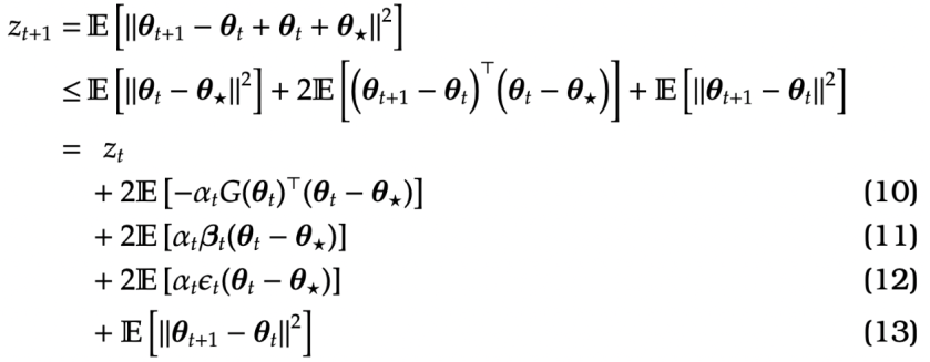
We now bound the four terms above.

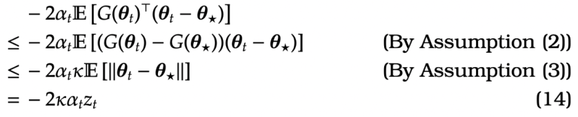
We can bound (10) as follows

$\begin{aligned} &-2\alpha_t \mathbb E \left[ G(\bm\theta_t)^\top (\bm\theta_t-\bm\theta_\star) \right] \notag \\ \leq \, & -2\alpha_t \mathbb E \left[ (G(\bm\theta_t) - G(\bm\theta_\star) ) (\bm\theta_t - \bm\theta_\star) \right] \tag{By Assumption \eqref{KW:As1}} \\ \leq \, & -2\alpha_t \kappa \mathbb E\left[ \left\| \bm\theta_t -\bm\theta_\star \right\| \right] \tag{By Assumption \eqref{KW:As2}} \\ =\, & -2 \kappa \alpha_t z_t \label{KW:eq1}\end{aligned}$ Screenshot 2022-10-28 at 10.54.36

For the term (11), by Cauchey-Schwartz

Screenshot 2022-10-28 at 10.55.31
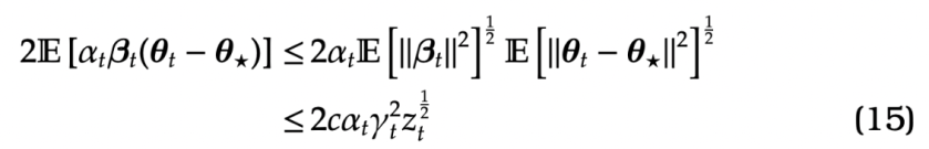
In the final inequality above we note that from Assumption (4) that: $\begin{aligned} \left\| \bm\beta_t \right\| := \left\| G(\bm\theta_t) - G_{\gamma_t} (\bm\theta_t) \right\| \leq c\gamma_t^2 \label{KW:eq3} %\end{aligned}$

Screenshot 2022-10-28 at 10.55.42

For term (12), we have $\begin{aligned} 2\mathbb E [ \alpha_t \bm\epsilon_t^\top (\bm\theta_t -\bm\theta_\star )] = 0 %\end{aligned}$

Screenshot 2022-10-28 at 10.57.09

because $\mathbb E[ \epsilon_t | \theta_{t} ]=0$ .

For term (13)

Screenshot 2022-10-28 at 11.01.17
Applying (14), (15), (16) and (17) to (10), (11) , (12) and (13) gives $\begin{aligned} z_{t+1} \leq z_t -2\kappa \alpha_t z_t + 2 c\alpha_t \gamma^2_t z_t^{\frac{1}{2}} + \frac{f_{\max}^2}{4} \frac{\alpha^2_t}{\gamma^2_t} %\end{aligned}$

Screenshot 2022-10-28 at 11.01.53

By the proposition above with $a_t = 2 \kappa \alpha_t$ , $b_t = c\gamma^2_t/\kappa$ and $e_t =\frac{f_{\max}^2}{4} \frac{\alpha_t}{\gamma^2_t}$ we see that $\begin{aligned} \limsup_{t\rightarrow \infty } \frac{z_t}{c^2\gamma_t^4/\kappa^2 + \alpha_t f_{\max}^2 / 4\gamma_t^2} \leq \frac{1}{2} %\end{aligned}$

Screenshot 2022-10-28 at 11.02.43

From this we see that the required result holds.

For $\alpha_t = {1}/{t}$ and $\gamma_t = {1}/{t^{1/6}}$ , we have

$\limsup_{t\rightarrow\infty} \frac{z_t}{t^{2/3}} \leq \frac{1}{2} \left[ \frac{c^2}{\kappa^2} +\frac{f_{\max}^2}{4} \right]$

which gives the final required expression. QED.

We now prove Proposition. We do so by proving Lemmas 1 and 2.

LEMMA 1. If $\xi_n$ is a positive sequence such that

$\xi_{n+1} \leq \xi_n \Big( 1- A \alpha_n\Big) + \alpha_n B$

and

$\sum_{n=1}^\infty \alpha_n = \infty, \qquad \limsup_{n\rightarrow\infty} \alpha_n \leq 0$

then

$\limsup_{n\rightarrow\infty} \xi_n \leq \frac{B}{A}\, .$

PROOF. Rearranging gives

$\xi_{n+1} - \xi_n \leq -\alpha_n (A \xi_n - B).$

If $\xi_n > B/A + \epsilon$ for some $\epsilon>0$ then

$\xi_{n+1} -\xi_n \leq -\alpha_n ( A \xi_n -B) \leq -\alpha_n ( A [B/A + \epsilon] -B) = -\alpha_n A \epsilon\, .$

So $\xi_n$ is decreasing when $\xi_n > B/A + \epsilon$ holds and, since $\sum_n \alpha_n = \infty$ , there exists $N$ s.t. $\xi_N \leq B/A +\epsilon$ . Let $N_0$ be the first value of $N$ where $\xi_N \leq B/A +\epsilon$ occurs.

Notice, $\xi_n$ can only increase when $\xi_n \leq B/A + \epsilon$ , and since $\xi_n$ is a positive then

$\xi_{n+1} \leq \xi_n + \alpha_n B\, .$

Thus, we see that

$\xi_n \leq \frac{B}{A} + \epsilon + \alpha_n A \epsilon , \qquad \forall n \geq N_0 \, .$

Therefore

$\limsup_{n\rightarrow\infty} \xi_n \leq \frac{B}{A} + \epsilon + \limsup_{n\rightarrow\infty} \alpha_n B \leq \frac{B}{A} + \epsilon \, .$

Since $\epsilon$ is arbitrary the results holds. QED.

LEMMA 2. If $\xi_n$ is a positive sequence such that

$\xi_{n+1} \leq \xi_n \Big( 1-A\alpha_n\Big) + \alpha_n \beta_n B$

and

$\sum_{n=1}^\infty \alpha_n = \infty, \qquad \lim_{n\rightarrow\infty} \alpha_n = 0, \quad \frac{\beta_n}{\beta_{n+1}} \leq \left( 1+C \alpha_n \right)$

with $A>C$ then

$\limsup_{n\rightarrow\infty} \frac{\xi_n}{\beta_n} \leq \frac{A-C}{B} .$

PROOF. Since $\lim_{n\rightarrow\infty} \alpha_n =0$ , take $N$ such that $\alpha_n < \delta$ for all $n \geq N$ .

Now defining $\xi'_n = \xi_n/\beta_n$ for $n\geq N$ gives

$\begin{aligned} \xi'_{n+1} = & \frac{\xi_{n+1}}{\beta_{n+1}} \leq \frac{\beta_n}{\beta_{n+1}} \Big( 1- A\alpha_n\Big) \xi_n' + \alpha_n \frac{\beta_n}{\beta_{n+1}} B \notag \\ \leq \, & \left( 1+C\alpha_n \right) \left( 1-A\alpha_n \right)\xi'_n + \alpha_n \left( 1+C\alpha_n \right)B\notag \\ \leq \, & \left( 1 -(A-C +\delta) \alpha_n \right)\xi'_n + \alpha_n (1+C \delta) B \notag \\ =\, & (1-A'\alpha_n) \xi'_n + \alpha_n B'\end{aligned}$

where we define $A' = A-C+\delta$ and $B'=(1+C\delta)B$ . Applying Lemma 1 gives

$\limsup_{n\rightarrow\infty} \xi'_n \leq \frac{A'}{B'} \, ,$

which recalling the definitions of $\xi_n'$ , $A'$ , $B'$ and recalling that $\delta$ is arbitrary gives the result. QED.

Proof of Proposition. By the inequality

$b_t z_t^{1/2} \leq \frac{z_t}{2} + \frac{b_t^2}{2} \,.$

we have

$\xi_{n+1} \leq \xi_n (1 -a_n/2) + a_n b^2_n + e_n a_n\, .$

Now the results follow by applying Lemma 2. With $\beta_n = b^2_n + e_n$ , $A= 1/2$ , $B=1$ and $C=0$ . (Notice we can take $C=0$ because $b_n$ and $e_n$ are decreasing.) QED.

References

The Kiefer-Wolfowitz procedure was first proposed by Kiefer and Wolfowitz (1952). Finite time bound similar to those in the Theorem above are given by Broadie et al. (2011). The analysis here largely follows from the arguments in Fabian (1967). Fabian and Broadie et al. both use results from Chung (1954), which is the basis for Lemmas 1 and 2 above.

Kiefer, J., & Wolfowitz, J. (1952). Stochastic estimation of the maximum of a regression function. The Annals of Mathematical Statistics, 462-466.

Broadie, M., Cicek, D., & Zeevi, A. (2011). General bounds and finite-time improvement for the Kiefer-Wolfowitz stochastic approximation algorithm. Operations Research, 59(5), 1211-1224.

Fabian, V. (1967). Stochastic approximation of minima with improved asymptotic speed. The Annals of Mathematical Statistics, 191-200.

Chung, K. L. (1954). On a stochastic approximation method. The Annals of Mathematical Statistics, 463-483.