Weighted Majority Algorithm

The Weighted Majority Algorithm is a randomized rule used to learn the best action amongst a fixed reference set.

We consider the following setting

There are a fixed set of actions $i=1,...,N$ which one may choose. There are a set of outcomes $y\in{\mathcal Y}$ .
After choosing an action $i$ , an outcome $y$ occurs and you receives a reward $r(i,y)\in [0,1]$ . Over time a policy $\pi$ chooses actions $\pi_t$ $t=1,...,T$ and outcomes $y_t$ , $t=1,...,T$ occur.
It is assumed that the function $r:\{1,...,N\}\times {\mathcal Y} \rightarrow [0,1]$ is known by the policy.
The accumulated a net reward is

$\rho(\pi,T):=\sum_{t=1}^T r(\pi_t,y_t).$

We are interested in how our dynamic policy $\pi$ performs in comparison to each fixed policy $i=1,...,N$ , that is a policy that chooses the same action $i$ at each time. In particular, we are interested in how this compares to the fixed policy which is retrospectively the best.

For this reason, we consider the regret of policy $\pi$

$R(\pi,T):=\max_{i=1,...,N}\left\{ \rho(i,T) -\bE \rho(\pi,T)\right\}.$

We can only retrospectively find the best fixed policy, whilst our policy $\pi$ must behave adaptively based on historical information. Thus $R(\pi,T)$ quantifies how we regret not having had the information to have chosen the best fixed policy.
Note a ‘good’ policy would have low regret. For instance, we might hope our dynamic policy is as good as the best fixed policy, i.e. $R(\pi,T)\leq 0$ .

Using Blackwell’s Approachability Theorem, we saw that low regret policies exist. See Section [Blackwell]Theorem [blackwell:regret]. One of the key advantages of such algorithms is that is does not place statistical assumptions on the outcome sequence $y_1,...,y_T$ . The Weighted Majority Algorithm is a further example of an algorithm that has asymptotically low regret and does not require statistical assumptions to be placed on the input sequence.

Weighted Majority Algorithm

For parameter $\eta>0$ , the \emph{(exponentially) weighted majority algorithm} is a randomized policy which chooses a policy $\latex i=1,…,N$ at time $t$ with probability $P(i,N)=\frac{1}{N}$ for $t=1$ and for $t\geq 1$

$P(i,t)=\frac{w_{i,t}}{W(t)},\qquad\text{where}\qquad w_{i,t}=e^{\eta\rho(i,t-1)} \quad\text{and}\quad W(t)=\sum_{i=1}^N e^{\eta \rho(i,t)}.$

We can derived the following regret bound

Theorem: If policy $\pi$ is the the weighted majority algorithm

(1) With $\eta$ fixed,

$\label{WMA:reg} \bE R(T) \leq \eta^{-1} \log(N) + \frac{\eta T}{2},$

for choice $\eta=\sqrt{2T^{-1}\log(N)}$ , the above bound states

$\label{WMA:reg2} \bE R(T) \leq 2\sqrt{2T \log(N)}.$

(2) For $\eta$ fixed the policy,

$\rho(\pi,T) \geq \frac{1 }{1-e^{-\eta}} \left\{ \eta \max_{i=1,...,N} \rho(i,T) +\log N\right\}.$

(3) For $\eta_t$ varrying over time and increasing, we have

$\label{WMA:reg} \bE R(T) \leq \eta_T^{-1} \log(N) + \frac{1}{8} \sum_{t=1}^T \eta_t,$

for choice $\eta_t=\sqrt{4t^{-1}\log(N)}$ , the above bound states

$\bE R(T) \leq \sqrt{ T \log N}$ •

Proof:

(1) Observe

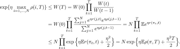
In the second inequaltiy, we apply the Azuma-Hoeffding Inequality, see Section [Azuma]. Taking logs and rearranging, we gain the required expression . Substituting $\eta=\sqrt{2T^{-1}\log(N)}$ , we gain expression .

(2) We note the following inequality holds

$\label{MWA:crude bound} \bE e^{\eta r(\pi_t,t)} \leq \bE [ (e^\eta -1)r(\pi_t,t) +1 ] \leq \exp\{ (e^{\eta}-1) \bE r(\pi_t,t)\}.$

In the first inequality, we bound with the line segment above the exponential. In the second inequality, we apply the bound $1+x\leq e^x$ . Applying bound to inequality , we have

$\exp\{\eta \max_{i=1,...,N} \rho(i,T)\} \leq N \prod_{t=1}^T \bE e^{\eta r(\pi_t,t)} \leq N \exp\{(e^{\eta}-1) \bE \rho(\pi,T) \}.$

Taking logs and rearranging gives the required bound.

(3) The crux of the proof (1) was that the function $N^{-1} W(T) \exp\{-\eta {\mathbb E} \rho(\pi,T) - \eta^2 T^2/2\}$ is decreasing and thus bounded above by $1$ . We apply the same prinicple, but we have to take account of the change in parameter $\eta_t$ .

We can express our weights differently, notice,

$\begin{aligned} \notag P(i,t)= \frac{\frac{1}{N}s_{i,t-1}^{\eta_t/\eta_{t-1}} }{\frac{1}{N} \sum_{j=1}^N s_{j,t-1}^{\eta_t/\eta_{t-1}}},\qquad \text{where}\qquad s_{i,t-1} & = \exp\left\{-\eta_{t-1} \rho(i,t-1) + \eta_{t-1} {\mathbb E} \rho(\pi, t-1) - \frac{1}{8}\eta_{t-1}\sum_{k=1}^{t-1} \eta_k \right\}\\ \text{and}\qquad\quad S(t) & = \frac{1}{N} \sum_{i=1}^N s_{i,t}.\notag \end{aligned}$

$S(t)^{\eta_t^{-1}}$ will play a similar role to that of $N^{-1} W(T) \exp\{-\eta {\mathbb E} \rho(\pi,T) - \eta^2 T^2/2\}$ in the proof of (1):

$\begin{aligned} S(t)^{\frac{1}{\eta_t}} % &\leq \left( \frac{1}{N} \sum_{j=1}^Ns_{j,t-1}^{{\eta_t}/{\eta_{t-1}}}\cdot e^{-\eta_t r(j,t) + \eta_t\bE r(\pi_t,t) - \frac{\eta_t^2}{8}} \right)^{\frac{1}{\eta_t}} \\ % & = \underbrace{\Bigg( \bE e^{-\eta_t r(\pi_t,t) + \eta_t (\bE r(\pi_t,t)) - \frac{\eta_t^2}{8}}\Bigg)^{\frac{1}{\eta_t}} }_{\leq 1, \text{ by Azzuma-Hoeffding}} \times \underbrace{ \left( \frac{1}{N} \sum_{j=1}^N s_{j,t-1}^{\eta_t/\eta_{t-1}}\right)^{\frac{1}{\eta_t}}}_{\leq S(t-1)^{\frac{1}{\eta_{t-1}}} \text{ by Jensen's Ineq}} \leq S(t-1)^{\frac{1}{\eta_{t-1}}} \end{aligned}$